Introduction
Researchers who work with smaller populations that have clearly defined boundaries (Laumann, Marsden, and Prensky 1989) may be able to design survey instruments that can feasibly document an entire social network. These complete, sociocentric networks can exhibit some systematic biases (Ready et al. 2020), but they typically do a better job of characterizing the full suite of direct and indirect connections within a population.
Many researchers, however, work in larger populations that have fuzzy boundaries, if any. In these settings it is usually not feasible to construct a complete social network using only a survey or semi-structured interview. An alternative approach is to collect egocentric networks from a random sample of individuals.
In this post, I will describe what an egocentric network is, and provide some simulation and sampling tools that can be used to understand the structural implications of an egocentric approach.
Egocentric networks
An egocentric network contains all of the alters connected to a particular ego (a single node), as well as all of the people to whom those ego’s alters are also connected. These two degrees of separation are sometimes referred to as the \(1^{st}\) and \(2^{nd}\) order neighborhoods of ego.
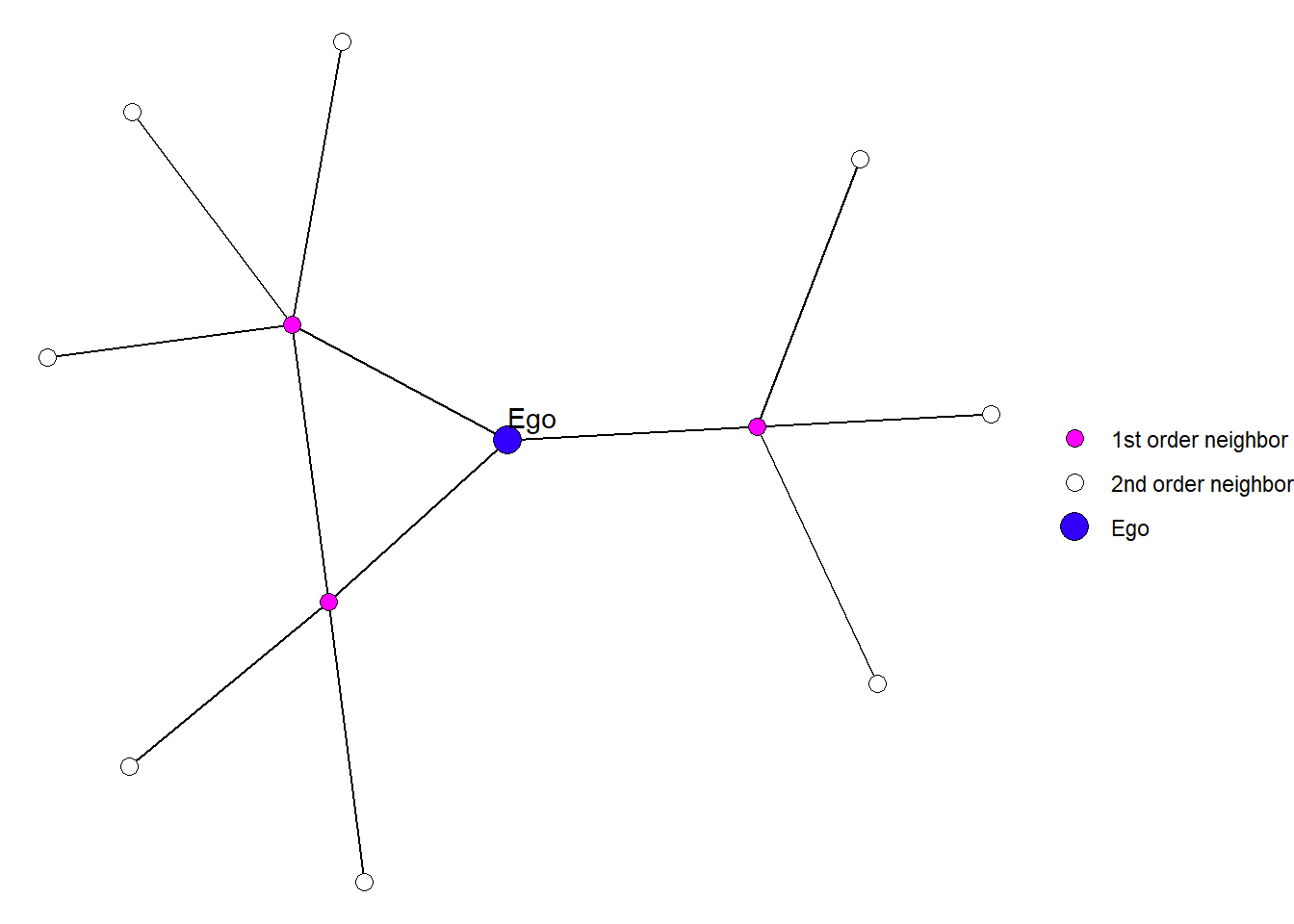
Figure 1: An example of an egocentric network.
Put differently, an egocentric design attempts to:
[observe] the network of interest from the point of view of a set of sampled actors, who provide information about themselves and anonymized information on their network neighbors (Krivitsky and Morris 2017: 1).
Look at the quote above, we can see that when we use an egocentric network design, we develop a survey instrument that asks survey respondents to do, at minimum, two network tasks.
First, we ask each ego to list the names of people with whom they have a particular relationship. In my work, I might ask people to list individuals with whom they have shared a meal in the past month. I might also ask them for details about the relationship, like how frequently they share meals, or how they are related to the person.
This procedure yields a short edgelist that might look something like this:
##   Node Edge Frequency Relation
## 1  Ego    A         3   friend
## 2  Ego    B         2   parent
## 3  Ego    C         2  sibling
## 4  Ego    D         5  sibling
## 5  Ego    E         3   friend
Once the respondent have listed their partners, the next steps is to ask them who those partners might also be connected with. For example, now that we know Ego has had a meal with person A, we will ask if they know who person A (and person B, etc.) has shared a meal with. We can also ask ego to estimate the frequency and how A is related to the person. In some cases, Ego might not know the answers to these questions.
##    Node Edge Frequency Relation
## 1     B    E         1   parent
## 2     B    F         3  sibling
## 3     B    G         2     <NA>
## 4     C    I         5   friend
## 5     C    J         3     <NA>
## 6     C    K         4  sibling
## 7     D    I         4  sibling
## 8     D    J         4 coworker
## 9     E    F         4  sibling
## 10    E    G         5     <NA>
These two edgelists represent the \(1^{st}\) and \(2^{nd}\) order neighborhoods of ego.
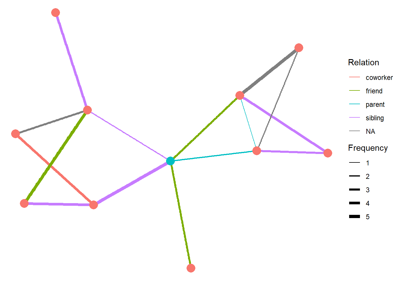
Figure 2: A graph of the hypothetical ego network described in the text above. Ego is shown in blue.
Limitations and benefits of egocentric networks
Observing a network through the lens of sampled egos presents has some limitations. Each respondent must be able to report information on themselves and all of their partners. For some relationships and details, this can be very challenging. The resulting network is also a biased representation of the complete network. This means that some centrality metrics – e.g., betweenness and closeness – are greatly affected by the incomplete network structure, while others – e.g., degree centrality – are less impacted (Marsden 2002).
But there are also some benefits that come from working with egocentric networks. A large amount of information can be obtained by only sampling a small number of people. This greatly reduces the amount of research effort needed to sample large populations. Egocentric networks also lend themselves to respondent driven sampling (Heckathorn 1997, 2002). Together these approaches can be used to document senstive or stigmatized social relations. Egocentric networks can also be constructed using contact diaries, which lend themselves to longitudinal network documentation (Fu 2007).
Egocentric sampling: A simulation study
So if you do work in a large population, and you intend to use an egocentric approach, you will be faced with some design questions:
- How many egos do you need to sample?
- What kinds of metrics will be biased?
- Can you conduct valid inferential statistics?
These questions are the focus of this simulation study. Here, I provide some tools you can use to simulate and visualize a sample of egos from a complete network and immediately see the ramifications. There are several packges used.
library(statnet)
library(igraph)
library(tidygraph)
library(ggraph)
library(ggforce)
library(patchwork)
library(intergraph)
egonetworks function
To begin, I’ve created a function that has several settings that can help you understand the implications of an egonetwork design. This is superficially similar to a power analysis used in statistical research design.
The overall purpose of the function is to simulate a complete network to use as a reference, and then sample egos from this complete network. By sampling egos and looking at their neighborhoods, we can get a sense of how the collection of egonetworks compare to the complete network structure.
egonetworks <- function(

  # SIMULATION SETTINGS
  N=30,
  directed = F,
  formula="net ~ edges + nodematch('group')",
  params=c(-3.5,3),
  groups = 4,

  # EGONETWORK SETTINGS
  select_egos=F,
  N_egos=3,
  egoIds,
  seed=777)

{

  # SIMULATE A COMPLETE NETWORK
  set.seed(seed)
  n <- N
  net <- network(n, directed = directed, density = 0)
  net %v% 'group' <- sample(1:groups, size = n, replace = T)
  g <- simulate(as.formula(formula), coef=params, seed = seed)

  # CONVERT TO IGRAPH
  ig <- asIgraph(g)

  # SAMPLE EGOS, FIND NEIGHBORHOODS
  if (select_egos == F) {
    egos <- sample(V(ig)$vertex.names, size=N_egos, replace = F)
    first <- ego(ig, order=1, nodes=egos, mindist = 0)
    second <- ego(ig, order=2, nodes=egos, mindist = 1)
  } else if (select_egos == T) {
    egos <- egoIds
    first <- ego(ig, order=1, nodes=egos, mindist = 0)
    second <- ego(ig, order=2, nodes=egos, mindist = 1)
  }

  # CREATE ATTRIBUTES
  tg <- ig %>%
    as_tbl_graph() %>%
    activate(nodes) %>%
    mutate(Neighborhood =  as.factor(ifelse( vertex.names %in% egos, 1,
                                             ifelse( vertex.names %in% unlist(first) | vertex.names %in% unlist(second), 2, 'Unobserved'))),
           egolab = ifelse( vertex.names %in% egos, paste('Ego', vertex.names), '' ),
           IsEgo = ifelse(vertex.names %in% egos, 'Yes','No')) %>%
    activate(edges) %>%
    mutate(Neighborhood = as.factor(ifelse(from %in% egos, 1,
                                           ifelse(to %in% egos, 1,
                                                  ifelse( from %in% unlist(first), 2,
                                                          ifelse( to %in% unlist(first), 2,  'Unobserved' ))))))

  # SAVE EGO NETWORKS
  E(ig)$id <- seq_len(ecount(ig))
  V(ig)$vid <- seq_len(vcount(ig))
  egographs <- make_ego_graph(ig,order=2,nodes=egos)

  # RETURN COMPLETE, TIDYGRAPH, AND EGONETWORKS IN A LIST
  return(list(g, tg, egographs))

}
The egonetworks function generates the following:
- One complete network.
- Node and edge attributes to visualize each egonetwork within the complete network.
- A list of egonetworks.
Simulation Settings
The function has the following default settings:
# SIMULATION SETTINGS
N=30,
directed = F,
formula="net ~ edges + nodematch('group')",
groups = 4,
params=c(-3.5,3),

# EGONETWORK SETTINGS
select_egos=F,
N_egos=3,
egoIds,
seed=777)
Simulation settings
N controls the number of nodes that are in the complete network simulation. directed controls whether the simulation generates a directed or undirected network.
egonetworks accepts a ergm formula that determines the structure for the network simulation. We covered ergm formulae in a previous post on network simulations with statnet. Currently, the default formula creates a network based on group membership homophily. The number of groups is controlled by the groups argument. But you can also include any ergm term in your formula, as long as the term does not require an attribute (see ?ergm-terms for details).
The params argument is used to specify parameters values that are required by the formula. Since the default formula is "net ~ edges + nodematch('group')", we need one parameter for network density (edges) and another for how strong the homophily is (nodematch). These parameters are specified in log-odds; log-odds = 0 is the same as 0.5 probability.
Egonetwork settings
Once a complete network is simulated from the settings above, we need to sample a number of egos from it. Here you have two options. If select_egos = FALSE, then you can set the number of egos to sample using N_egos. The number of egos you choose will be randomly sampled from the nodes in the complete network (based seed). Alternatively, if select_egos = TRUE, you can provide a vector of egoIds. This is useful if you want to take a deep examinations of a specific node.
Testing it out
You can run egonetworks with just the defaults and a list will be generated. The first element of the list is the complete network as a network object.
test <- egonetworks()
test[[1]]
##  Network attributes:
##   vertices = 30
##   directed = FALSE
##   hyper = FALSE
##   loops = FALSE
##   multiple = FALSE
##   bipartite = FALSE
##   total edges= 54
##     missing edges= 0
##     non-missing edges= 54
##
##  Vertex attribute names:
##     group vertex.names
##
## No edge attributes
The second element is a tbl_graph object with node and edge attributes that can be used for visualization.
test[[2]]
## # A tbl_graph: 30 nodes and 54 edges
## #
## # An undirected simple graph with 2 components
## #
## # Edge Data: 54 x 4 (active)
##    from    to na    Neighborhood
##   <int> <int> <lgl> <fct>
## 1     1     6 FALSE 2
## 2     1     9 FALSE 1
## 3     1    11 FALSE 1
## 4     1    14 FALSE 2
## 5     1    27 FALSE 2
## 6     1    30 FALSE 2
## # ... with 48 more rows
## #
## # Node Data: 30 x 6
##   group na    vertex.names Neighborhood egolab IsEgo
##   <int> <lgl> <chr>        <fct>        <chr>  <chr>
## 1     2 FALSE 1            2            ""     No
## 2     4 FALSE 2            2            ""     No
## 3     4 FALSE 3            2            ""     No
## # ... with 27 more rows
And the third element is a list of igraph objects based on all the ego graphs that were subset by make_ego_graph.
test[[3]]
## [[1]]
## IGRAPH 22e6c59 U--- 20 37 --
## + attr: group (v/n), na (v/l), vertex.names (v/c), vid (v/n), na (e/l),
## | id (e/n)
## + edges from 22e6c59:
##  [1]  1-- 5  1-- 8  1-- 9  1--11  1--17  1--20  2-- 8  2-- 9  2--10  2--15
## [11]  3-- 5  3-- 6  4-- 7  4--19  5-- 6  5-- 8  5--15  5--16  5--17  5--18
## [21]  6--12  6--17  6--18  7-- 8  7--12  7--19  8--14  8--18  9--16 10--11
## [31] 10--15 11--16 13--14 14--17 14--18 16--18 17--20
##
## [[2]]
## IGRAPH 22e6c59 U--- 14 26 --
## + attr: group (v/n), na (v/l), vertex.names (v/c), vid (v/n), na (e/l),
## | id (e/n)
## + edges from 22e6c59:
##  [1]  1-- 4  1-- 5  3-- 5  4-- 5  1-- 6  3-- 6  2-- 7  6-- 7  2-- 8  3-- 8
## [11]  7-- 8  1-- 9  8-- 9  3--10  4--10  8--10  4--11  6--11  9--11  1--12
## [21]  4--12  4--13  5--13 11--13  1--14 12--14
##
## [[3]]
## IGRAPH 22e6c59 U--- 14 23 --
## + attr: group (v/n), na (v/l), vertex.names (v/c), vid (v/n), na (e/l),
## | id (e/n)
## + edges from 22e6c59:
##  [1]  1-- 3  3-- 4  1-- 6  2-- 6  3-- 6  5-- 6  6-- 8  7-- 8  7-- 9  7--10
## [11]  9--10  3--11  1--12  3--12  4--12  8--12  3--13  4--13  6--13  8--13
## [21] 11--13  1--14 12--14
Visualization
First, let’s take a look at what the complete network looks like for a few different seed values.
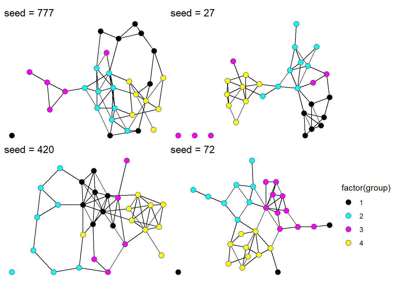
Figure 3: Complete undirected networks for four different seed values.
Coloring each node by group membership, we see how our simulation has generated a network based on group homophily.
The default settings draw three egos randomly out of the thirty used in the simulation. We can use the Neighborhood and IsEgo variables to color the edges and nodes. These variables tag which nodes and edges are part of the \(1^{st}\) and \(2^{nd}\) degree neighborhoods and which nodes are unobserved (Neighborhood = 0). The egolab variables can be used to label each ego.
Let’s focus on seed = 777 and seed = 72.
p1 <- egonetworks(seed = 777)[[2]] %>%
  ggraph() +
  geom_edge_link0(aes(color=Neighborhood)) +
  geom_node_point(aes(color=Neighborhood, shape=IsEgo), size=2) +
  geom_node_label(aes(label=egolab), repel = T) +
  theme_void() + theme(legend.position = 'none') +
  scale_edge_color_manual(values=c('#3300ff','magenta','#00000033')) +
  scale_color_manual(values=c('#3300ff','magenta','#00000033')) +
  ggtitle('seed = 777')

p2 <- egonetworks(seed = 72)[[2]] %>%
  ggraph() +
  geom_edge_link0(aes(color=Neighborhood)) +
  geom_node_point(aes(color=Neighborhood, shape=IsEgo), size=2) +
  geom_node_label(aes(label=egolab), repel = T) +
  theme_void() + #theme(legend.position = 'none') +
  scale_edge_color_manual(values=c('#3300ff','magenta','#00000033')) +
  scale_color_manual(values=c('#3300ff','magenta','#00000033')) +
  ggtitle('seed = 72')

p1 + p2
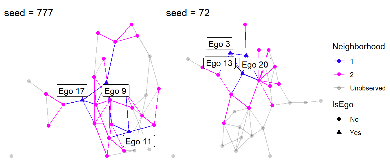
Figure 4: Visualizing egocentric networks.
Looking at Figure 4, something clearly stands out. Can you tell what it is?
A sample of three egos is capable of recovering a lot of the complete network structure, but only if those egos occupy different structural positions in the network. This is somewhat true when we used seed = 777, but seed = 72 happened to select three nodes that are all connected to each other. This greatly reduces the our ability to observe the complete network.
It is easy to notice this when we have the complete network already. But how would we know this if we haven’t and cannot collect a complete network?
One approach is to used stratified random sampling instead of purely random sampling. This requires that we have some background, contextual knowledge of the populationwe are studying. For instance, if we know that there are a number of organization in the population, we need to be sure to sample egos from each of them. In our simulation study, this means we need to sample at least one ego from each of our homophily groups.
Similarly, if we have reason to believe that a person’s position in a network is correlated with other personal attributes (e.g., wealth, age, location), then we can take stratified random samples of people who have different attributes.
A larger network
Now that we have a sense of how this function behaves, let’s take it up a notch.
In reality, you probably wouldn’t use an egocentric approach for a population of 30. More likely you’d what to use it for a much large population, say, 500 nodes. Let’s parameterize this.
First, we need to build some intuition. Start by simulating a network with 500 nodes using the default params and then calculating the density on the complete network.
eg <- egonetworks(N = 500)
graph.density(asIgraph(eg[[1]]))
## [1] 0.03502204
This is much too dense. Most real world networks are more sparse – a topic I discuss in this blog post. The sparsepoint for a network with 500 nodes is:
sparsepoint <- function(n, directed=F) {
  if ( directed == F  )   { n / (n*(n-1)/2) }
  else if ( directed == T ) { n / (n*(n-1))   }
  else {
    print('Must be TRUE or FALSE.')
  }
}

sparsepoint(500, directed = F)
## [1] 0.004008016
So to improve the simulation, we should set more extreme params.
eg <- egonetworks(N = 500, params = c(-8,4))
graph.density(asIgraph(eg[[1]]))
## [1] 0.004857715
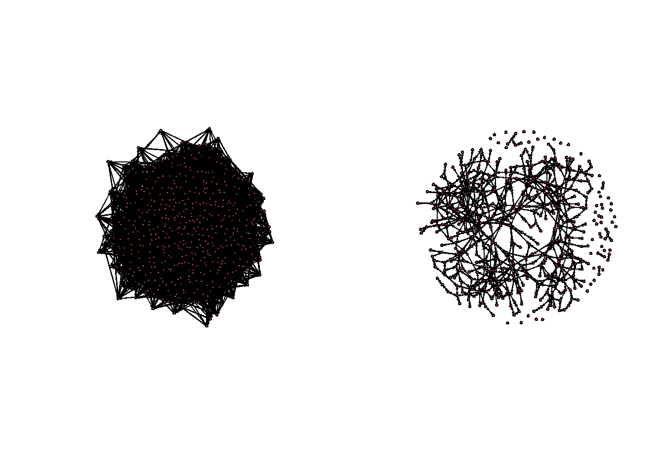
Much better. The visual difference is striking.
par(mfrow=c(1,2))
gplot(egonetworks(500, params = c(-3.5,3))[[1]] )
gplot(egonetworks(500, params = c(-8,4))[[1]])
Now that we have some more reasonable parameters, let’s sample different quantities of N_egos and see how well we recover the complete network. We’ll try 3,10,35, and 60. For brevity, I’ve omitted the plotting code, but an example is show below.
params <- c(-8,4)
mypal <- c('#3300ff','magenta','#00000033')

p1 <-
  egonetworks(
    N=500,
    params = params,
    N_egos = 3)[[2]] %>%
  ggraph() +
  geom_edge_link0(aes(color=Neighborhood)) +
  geom_node_point(aes(color=Neighborhood, shape=IsEgo), size=1.5) +
  theme_void() + theme(legend.position = 'none') +
  scale_edge_color_manual(values=mypal) +
  scale_color_manual(values=mypal) +
  ggtitle('N_egos = 3')
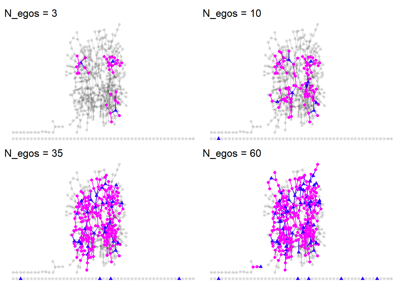
As we increase the number of egos, we get much closer to the complete network. We also end up smapling some isolates by chance. But this qualitative approach isn’t all that satisfying. We need to make some quanitative comparisons between the complette network and the merged egocentric networks.
To do this, we first need to take all of the egonetworks, (i.e., egonetworks()[[3]]) and combine them into a single network. Then we will look at how the structural characteristics compare between the complete and egocentric versions.
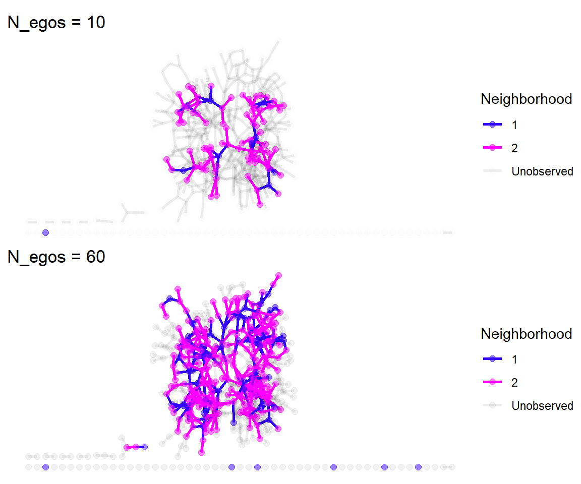
Merging the egonetworks
There may be some fancy igraph ways to combine these networks, but I think the most straight forward approach is to get the edgelist for every network, using rbind to combine them, and then eliminate any duplicate edges.
I’m going to do this once with 10 egos and once with 60 egos. Since each egonetwork is stored in a list, I’ll use lapply to get.edgelist and converted all the edgelists into data.frame so that they can be unlisted using dplyr::bind_rows.
params <- c(-8,4)
egonet10 <- egonetworks(N=500, params = params, N_egos = 10)[[3]]
egonet60 <- egonetworks(N=500, params = params, N_egos = 60)[[3]]

# add names to egonetworks
for(i in seq_along(egonet10)) {
  V(egonet10[[i]])$name <- V(egonet10[[i]])$vid
}
for(i in seq_along(egonet60)) {
  V(egonet60[[i]])$name <- V(egonet60[[i]])$vid
}

# get edgelists
el10 <- dplyr::bind_rows(
  lapply(
    lapply(egonet10, get.edgelist), as.data.frame) )
el60 <- dplyr::bind_rows(
  lapply(
    lapply(egonet60, get.edgelist), as.data.frame) )

# graph the edgelist without duplicates
g10 <- graph.data.frame(el10[ !duplicated(el10), ])
g60 <- graph.data.frame(el60[ !duplicated(el60), ])
Network comparisons
How do network statistics calculated on the compiled egonetworks compared to the full network?
##    Network N_nodes     Density AvgPathLength Connectedness
## 1 Complete     500 0.004857715      7.705835     0.7498677
## 2   60Egos     289 0.004060938      1.775687     0.9793829
## 3   10Egos      91 0.010866911      1.617834     0.3789988
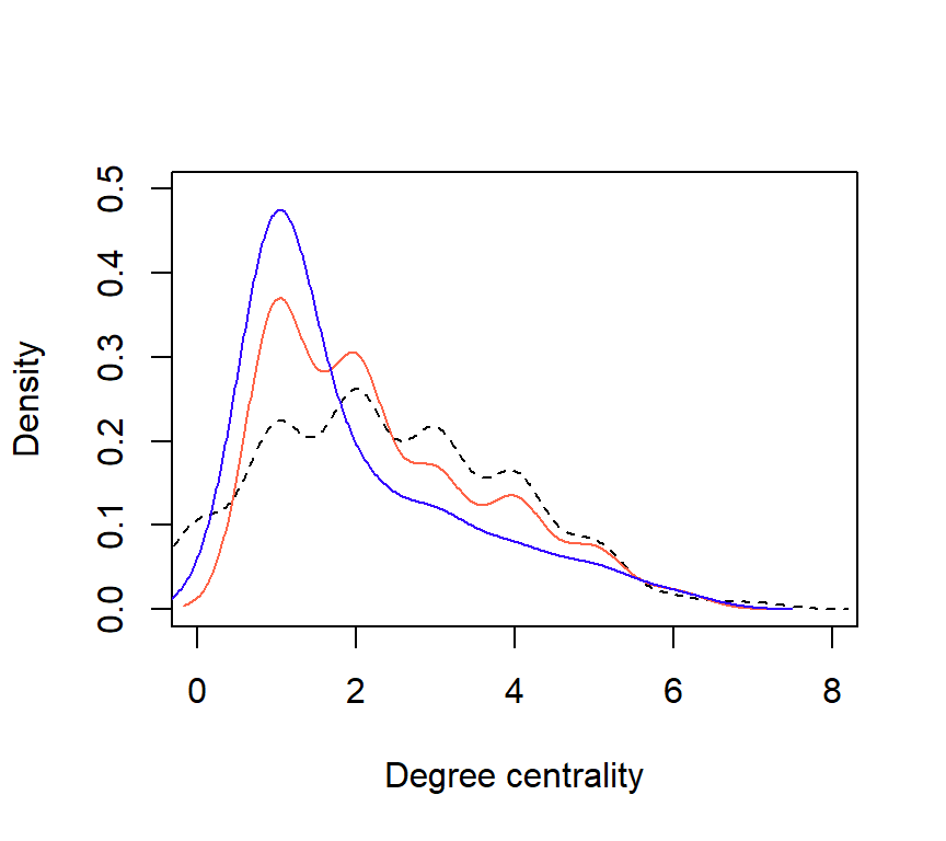
Figure 5: Comparison of degree distributions for each network (Complete = dashed; 60Egos = orange; 10Egos = purple.
Concluding thoughts
- Egocentric networks are capable of estimating the structure of large networks with much lower research effort.
- Network simulation and the
egonetworksfunction are tools for anticipating how much research effort is needed. They can be used like a power analysis. - Theory and ethnographic knowledge is necessary for adequate research design, but relatively little prior knowledge is needed to come up with useful simulations.
We have not touched on inferential statistics with ego.ergm but this package is very useful for developing statistically models on egocentrically sampled data. We will cover this in a future post.
References
Fu, Yang-chih. 2007. “Contact Diaries: Building Archives of Actual and Comprehensive Personal Networks.” Field Methods 19 (2): 194–217.
Heckathorn, Douglas D. 1997. “Respondent-Driven Sampling: A New Approach to the Study of Hidden Populations.” Social Problems 44 (2): 174–99.
———. 2002. “Respondent-Driven Sampling II: Deriving Valid Population Estimates from Chain-Referral Samples of Hidden Populations.” Social Problems 49 (1): 11–34.
Krivitsky, Pavel N, and Martina Morris. 2017. “Inference for Social Network Models from Egocentrically Sampled Data, with Application to Understanding Persistent Racial Disparities in HIV Prevalence in the US.” The Annals of Applied Statistics 11 (1): 427.
Laumann, Edward O, Peter V Marsden, and David Prensky. 1989. “The Boundary Specification Problem in Network Analysis.” Research Methods in Social Network Analysis 61: 87.
Marsden, Peter V. 2002. “Egocentric and Sociocentric Measures of Network Centrality.” Social Networks 24 (4): 407–22.
Ready, Elspeth, Patrick Habecker, Roberto Abadie, Carmen A Dávila-Torres, Angélica Rivera-Villegas, Bilal Khan, and Kirk Dombrowski. 2020. “Comparing Social Network Structures Generated Through Sociometric and Ethnographic Methods.” Field Methods 32 (4): 416–32.