Introduction
We can a learn a lot about a network using visualization tools and descriptive statistics. But many researchers would like to make inferences about how specific variables influence the probability of a network connection. There are multiple ways to do this – latent network modeling, multilevel Bayesian models, quadratic assignment procedures – but one of the most common and versatile methods is to build Exponential Random Graph Models (ERGMs).
To start learning ERGMs, we will use the statnet suite of packages, one of which is the ergm package. Let’s begin by installing statnet.
#install statnet suite
#install.packages('network', dependencies = T)
#install.packages('statnet', dependencies = T)
library(statnet)
What is an ERGM?
ERGMs are used to model the structural dependencies in a relational data object. For our purposes, these dependencies are the edges between the nodes and we can use an ERGM to estimate both the probability and uncertainty that such an edge exists in a given graph. More conventional statistical approaches fail in this endeavor because they assume that observations are independent, and we are specifically interested in the dependence of our observations.
In essence, an ERGM is used to model the likelihood of an edge between each pair of nodes. In this sense, an ERGM is a dyadic model (Morris, Handcock, and Hunter 2008). There are many different types of ERGMs. Each variation is used to model networks with different kinds of edges, for instance:
- Binary ERGMs are for edges that are present or absent.
- Valued ERGMs (VERGMs) are for weighted networks; edges > 1.
- Temporal ERGMs (TERGMs) for longitudinal networks; edges turn on and off over time.
- Bayesian ERGMs (BERGMs) for probabilistic networks; edges are probabilities.
In the examples to follow, we will be working with a binary ERGM.
Why use ERGMs?
There are many other approaches for studying data structures in which the observations are not independent of each other. So why should we use ergms? One of the greatest advantages of ERGMs is the ability to include structural elements of networks as predictive terms in a model.
For instance, we have discussed the role of triadic closure in the formation of networks. Using ERGMs we can include a triangle predictor that will tell us how well triangles described the pattern of connections in a network.
There are many ERGM terms, each representing a different configurations of links in a network. You can learn about them by calling ?ergm-terms. We will use some of these today, but we will focus on them more in our next meeting. We also encourage to read the “Specification of Exponential-Family Random Graph Models: Terms and Computational Aspects” by Morris, Handcock, and Hunter (2008). A link to this paper is located on our website Canon under Network Modeling.
Getting started
Today we are going to be analyzing how fishing households share their catch with other households. Let’s start by loading in the edgelist and the household attributes. This file is available on the SENG github.
net = readRDS('fishing_network.Rdata')This is a binary, directed network. An directed edge between two nodes in this network indicates that one household has shared a portion of their catch with another household. Let’s examine the network object.
net## Network attributes:
## vertices = 67
## directed = TRUE
## hyper = FALSE
## loops = FALSE
## multiple = FALSE
## bipartite = FALSE
## total edges= 272
## missing edges= 0
## non-missing edges= 272
##
## Vertex attribute names:
## family harvest hhsize owner vertex.names
##
## No edge attributesWe see that there are 67 households in this network with a total of 272 edges between them. The density of this network is 0.0615106, which indicates that it is relatively sparse.
This network has five vertex attributes that we added to the network using the hh_attributes.csv file. One of these in an id used for each vertex name. The second variable, harvest, is a standardized measure of the size of the households catch. The third column is a standardized measure of the household size. These variables have been standardized so that they can be compared directly in our models.
Finally, The owner variable indicates whether or not that household owns a boat to use for fishing, and the final column is a grouping variable which indicates which family the household is a part of; these families are coded as A through D.
Research questions
Before we dig into the ERGMs, let’s state some clear question that we will use to guide our analysis. Based on previous studies of fishing communities, we should ask the following questions:
- Kinship – Are households from the same family more likely to share with each other?
- Reciprocity – Are sharing connections more likely when the relationship is reciprocal?
- Surplus and productivity – Do households with large harvests tend to have more sharing relationships? Are households with small harvests likely to be recipients?
Visualizing the network might give us some qualitative clues about the answers of these questions. Let’s create a graph where each node is colored by it’s family group. Then we will resize each node according to the size of it’s harvest, and highlight reciprocity edges.
A full description of visualization techniques is beyond the scope of this meeting, so for brevity I’ll just say that I am going to use igraph, tidygraph, and ggraph to create this visual. The code is shown below.
library(igraph)
library(tidygraph)
library(ggraph)

gnet = intergraph::asIgraph(net)
E(gnet)$mutual = is.mutual(gnet)

as_tbl_graph(gnet) %>%
    ggraph() +
    theme_void() +
    geom_edge_link(aes(color=mutual), width=0.9, alpha=0.75,
                   arrow = arrow(length=unit(2, 'mm')), end_cap=circle(3,'mm')) +
    geom_node_point(aes(fill=family, size=harvest), pch=21) +
    scale_size_continuous(range = c(0.5,8)) +
    scale_fill_viridis_d() +
    scale_edge_color_manual(values = c('grey50','tomato'))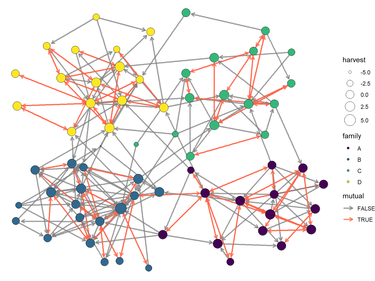
The graph above seems to suggest that there are some family clusters and possibly that reciprocity is more common between family members. But other than that, there is little else that we can understand from just looking at the graph. This is why we need ERGMs!
ERGM syntax
When you run a linear regression in R, the typical syntax looks something like this:
y ~ 1 + x1 + x2
In this syntax, the tilde indicates that we modeling the outcome variable y as a function of the intercept 1 and the variables x1 and x2. The output of a model like this will be an estimate of the Intercept and a two beta coefficients that represent the effect that x1 and x2 have on y.
In a ERGM, we using a simlar syntax:
net ~ edges + …
In this syntax, our network object is the outcome, and we model it as a function of the edges term and some other ergm-terms … The edges term behavior very similarly to the intercept in a regression, although the interpretation is slightly different. Whereas an intercept provides an estimate of the mean value of y when all variables are set to 0, the edges term tells us the network density when all terms are set to 0.
Let’s run our first ergm to show that this is true.
fit0 = ergm(net ~ edges)## Starting maximum pseudolikelihood estimation (MPLE):## Evaluating the predictor and response matrix.## Maximizing the pseudolikelihood.## Finished MPLE.## Stopping at the initial estimate.## Evaluating log-likelihood at the estimate.summary(fit0)## Call:
## ergm(formula = net ~ edges)
##
## Maximum Likelihood Results:
##
## Estimate Std. Error MCMC % z value Pr(>|z|)
## edges -2.72506 0.06259 0 -43.54 <1e-04 ***
## ---
## Signif. codes: 0 '***' 0.001 '**' 0.01 '*' 0.05 '.' 0.1 ' ' 1
##
## Null Deviance: 6130 on 4422 degrees of freedom
## Residual Deviance: 2044 on 4421 degrees of freedom
##
## AIC: 2046 BIC: 2052 (Smaller is better. MC Std. Err. = 0)Our estimate for the density is -2.7250615. This seems pretty different from the network density we calculated above: 0.0615106. This is because binary ERGMs report coefficient on the log-odds scale. On this scale, a value of 0 is the same as a 0.5 probability.
To check our density estimates, we need to convert log-odds to probability. We do this by converting log-odds to an odds-ratio…
odds = exp(coef(fit0))
odds
## edges
## 0.06554217and then dividing the odds by (1 + odds).
odds / (1 + odds)## edges
## 0.06151063Compare this to the network density
network.density(net)## [1] 0.06151063To simplify this process for later on, let’s write a function.
logit2prob = function(x) {
    odds = exp(x)
    prob = odds / (1 + odds)
    return(prob)
}
Now that we are equipped with an understanding of log-odds and probability, let’s starting tackling question 1.
Question 1
In this question, we want to know if households from the same family are more likely to share with one another. This is a form of family homophily. We can model this process by including a nodematch term from the archive of ergm-terms.
nodematch calculates the log-odds of an edge when two nodes match on a particular attributes. The syntax looks like this:
net ~ edges + nodematch(‘family’).
We include the name of the variables within the parenthesis following nodematch. This is a common structure in other ergm-terms as well. Let’s run it.
fit1.1 = ergm(net ~ edges + nodematch('family'))## Starting maximum pseudolikelihood estimation (MPLE):## Evaluating the predictor and response matrix.## Maximizing the pseudolikelihood.## Finished MPLE.## Stopping at the initial estimate.## Evaluating log-likelihood at the estimate.From the read out, we learn that this ERGM is using maximum pseudolikelihood estimation to estimate this effect. Let’s examine the model summary.
summary(fit1.1)## Call:
## ergm(formula = net ~ edges + nodematch("family"))
##
## Maximum Likelihood Results:
##
## Estimate Std. Error MCMC % z value Pr(>|z|)
## edges -4.8134 0.1932 0 -24.91 <1e-04 ***
## nodematch.family 3.5993 0.2065 0 17.43 <1e-04 ***
## ---
## Signif. codes: 0 '***' 0.001 '**' 0.01 '*' 0.05 '.' 0.1 ' ' 1
##
## Null Deviance: 6130 on 4422 degrees of freedom
## Residual Deviance: 1466 on 4420 degrees of freedom
##
## AIC: 1470 BIC: 1482 (Smaller is better. MC Std. Err. = 0)Just like a regression, we get an estimate of the Standard Error. When the Std. Error is greater than the estimate, this is an indication that the effect is uncertain. However, in this case we have a clear positive effect of family homophily. This is reinforced by the low p-value.
Let’s calculate the odds.
exp(coef(fit1.1))## edges nodematch.family
## 0.008120301 36.571268229This tells us that an edge is 36.5712682 times more likely if two nodes come from the same family. That is a strong effect. If we want to express this in probability, then we need to add the coefficients together.
# multiply coef[2] by 1 for nodematch = T
logit2prob(coef(fit1.1)[1] + coef(fit1.1)[2]*1)
## edges
## 0.228972Taking the low density into account, an edge between two households in the same family is 0.228972. A somewha low probability, but not nearly as low as it is for two nodes from different families.
# multiply coef[2] by 0 for nodematch = F
logit2prob(coef(fit1.1)[1] + coef(fit1.1)[2]*0 )
## edges
## 0.008054893Goodness-of-fit
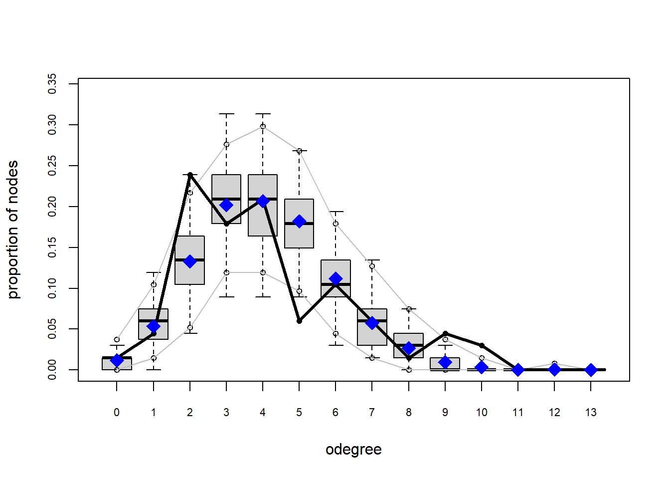
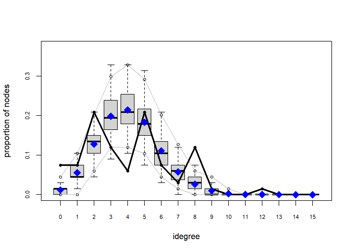
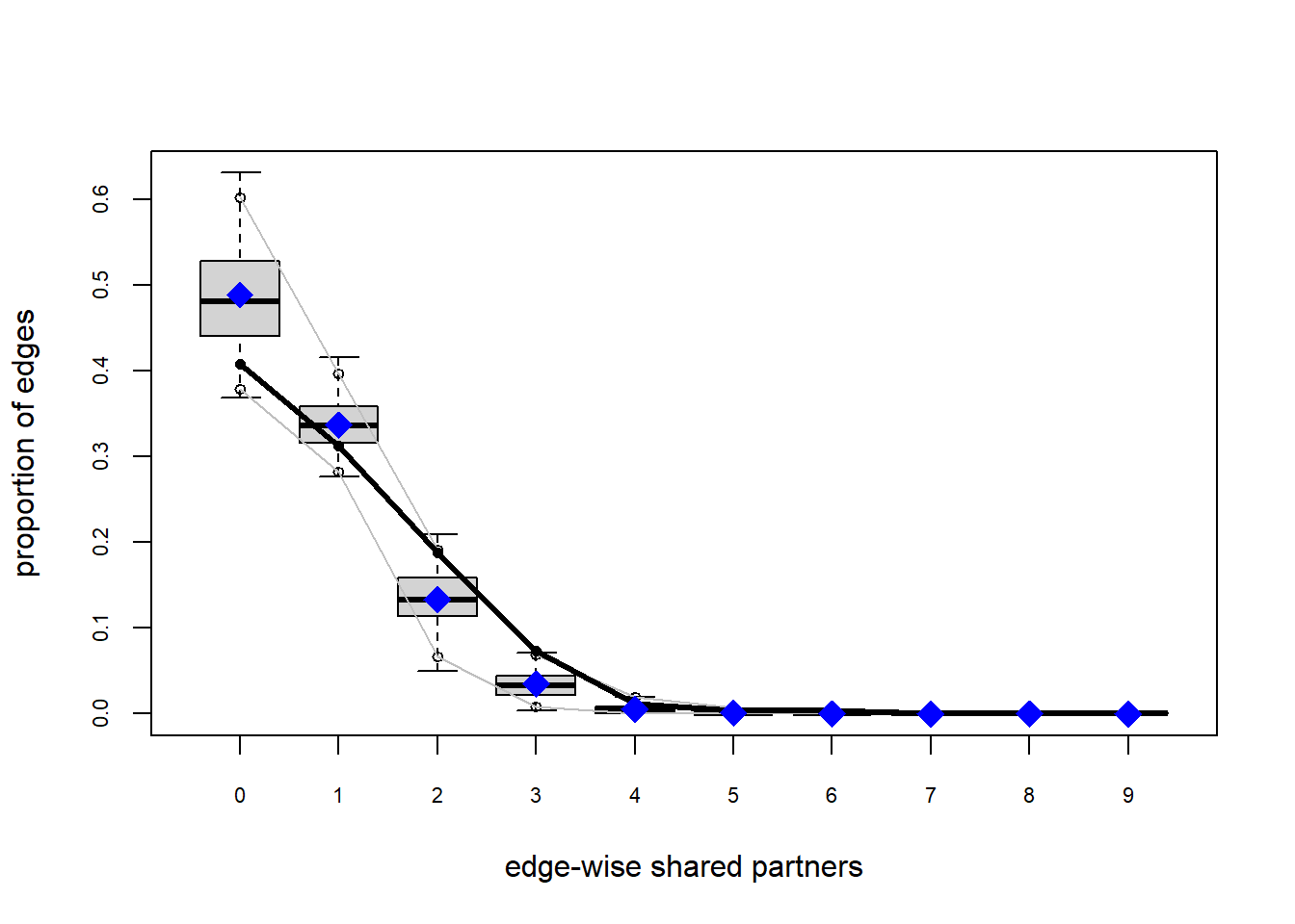
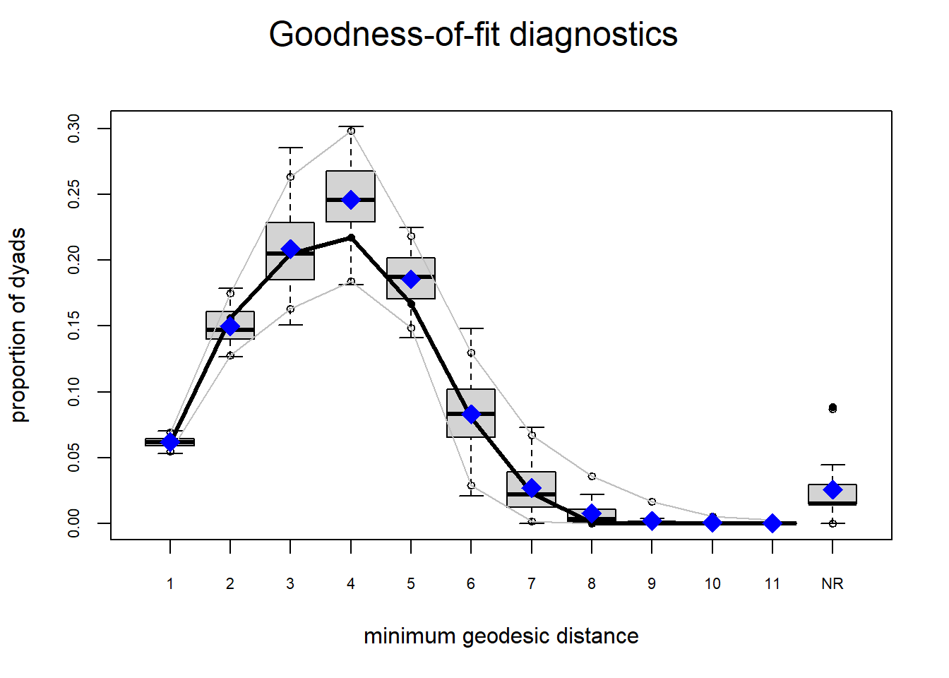
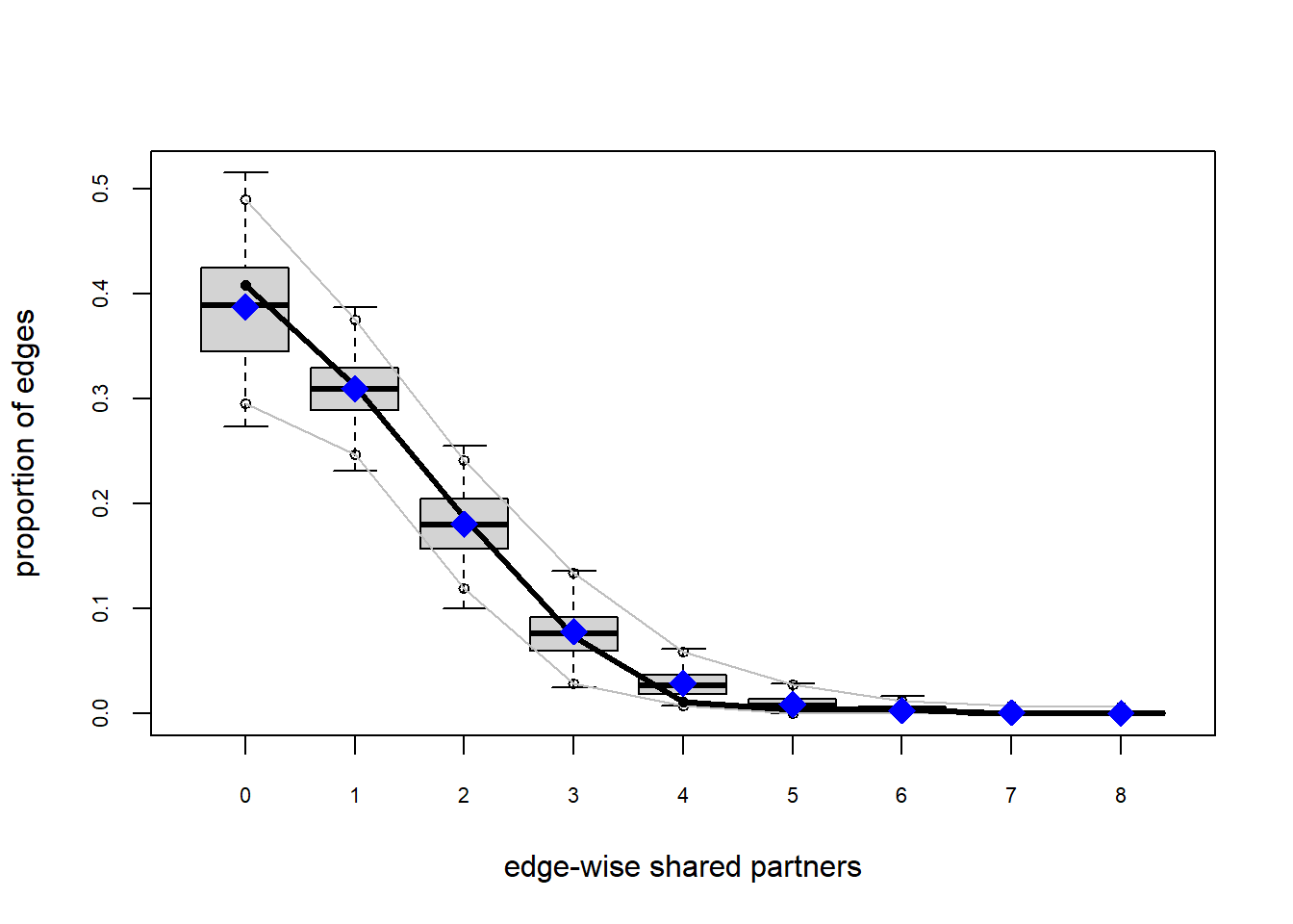
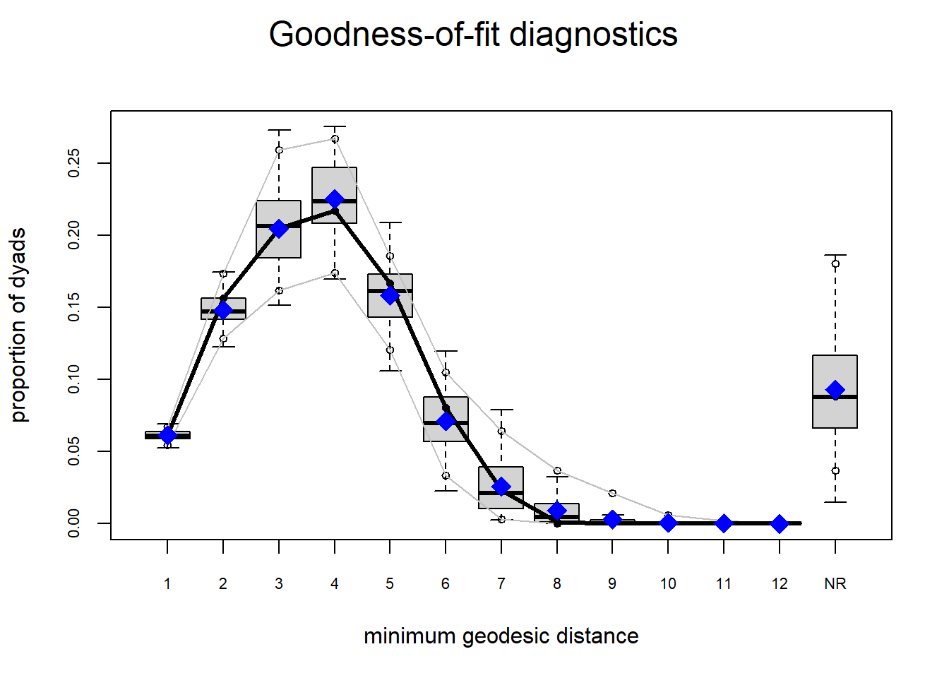
One way that we can test how well this model describe our data is by assessing the Goodness-of-fit. ergm comes with a convenient gof function that does this. If we plat it within the plot function, we receive some diagnostic plots.
plot(gof(fit1.1))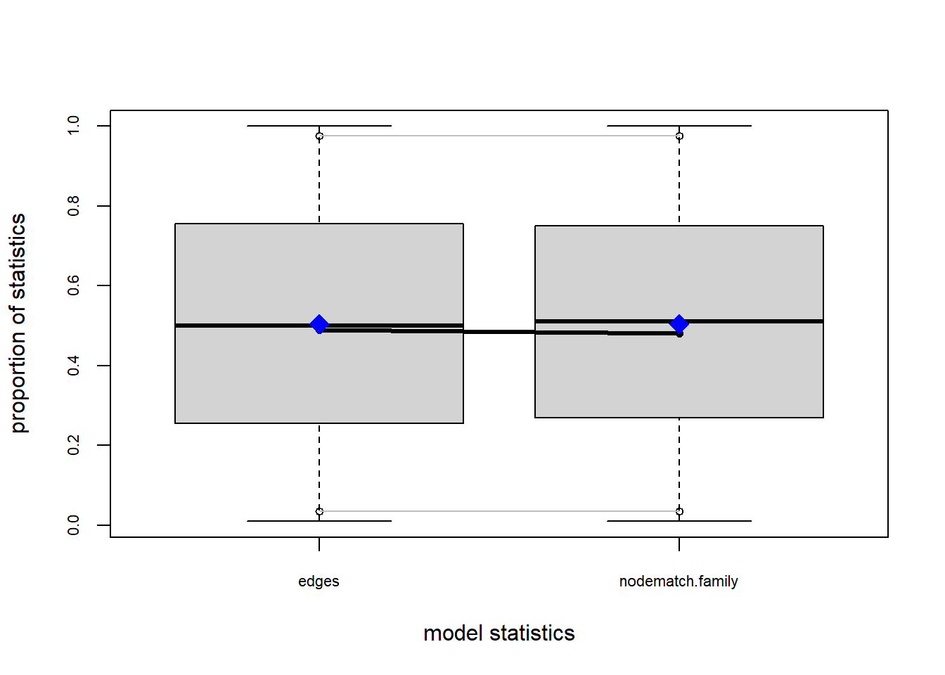
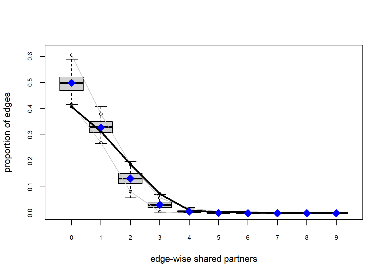
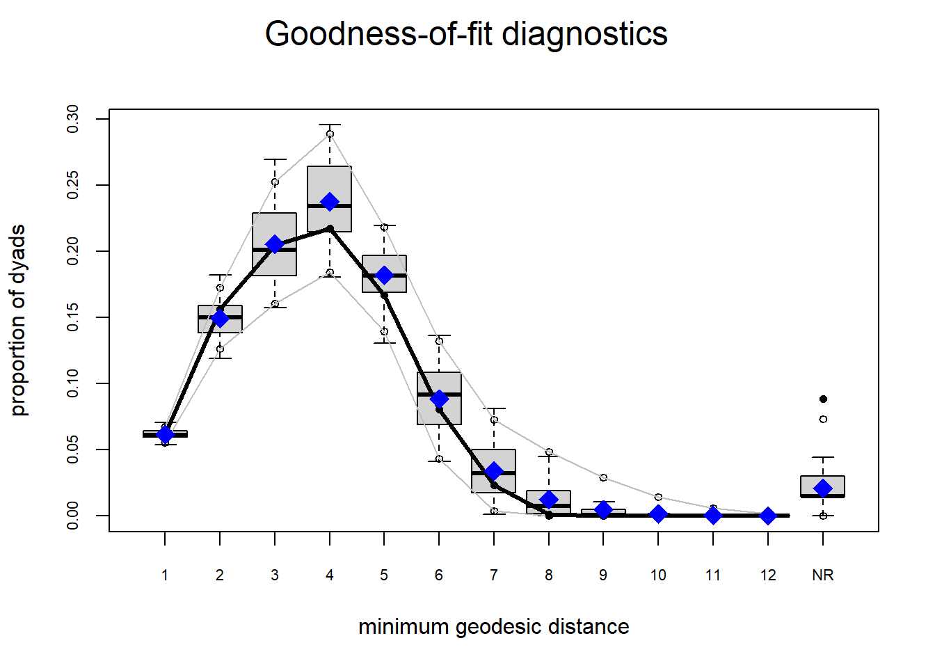
The gof function uses our ergm coefficients to simulate thousands of networks. It then calculates a set of descriptive statistics on each simulated network and compares the distribution of these statistics to the observed values. The observed values on plotted on each graph as a black line.
Looking at the diagnostics, we see that our model does not capture the distribution of in-degree and out-degree very well (plots 2 and 3). However, this model closely resembles values of edgewise shared partners and slightly overestimates values of minimum geodesic distance.
These mismatches are likely because there are other aspects of the network formation process beyond homophily.
Question 2
This brings us to our second question: is sharing more likely if relationships are reciprocated? To test this, we need to use the mutual term. The mutual term estimates the log-odds of an edge from i to j if there is an existing edge from j to i.
The mutual term has some other options. We can estimate reciprocity for specific attributes. For now, we will look at reciprocity in general.
fit2.1 = ergm(net ~ edges + mutual)## Starting maximum pseudolikelihood estimation (MPLE):## Evaluating the predictor and response matrix.## Maximizing the pseudolikelihood.## Finished MPLE.## Starting Monte Carlo maximum likelihood estimation (MCMLE):## Iteration 1 of at most 60:## Warning: 'glpk' selected as the solver, but package 'Rglpk' is not available;
## falling back to 'lpSolveAPI'. This should be fine unless the sample size and/or
## the number of parameters is very big.## Optimizing with step length 1.0000.## The log-likelihood improved by 0.4608.## Estimating equations are not within tolerance region.## Iteration 2 of at most 60:## Optimizing with step length 1.0000.## The log-likelihood improved by 0.0024.## Convergence test p-value: 0.2944. Not converged with 99% confidence; increasing sample size.
## Iteration 3 of at most 60:
## Optimizing with step length 1.0000.
## The log-likelihood improved by 0.0393.
## Convergence test p-value: 0.0642. Not converged with 99% confidence; increasing sample size.
## Iteration 4 of at most 60:
## Optimizing with step length 1.0000.
## The log-likelihood improved by 0.0609.
## Convergence test p-value: 0.0090. Converged with 99% confidence.
## Finished MCMLE.
## Evaluating log-likelihood at the estimate. Fitting the dyad-independent submodel...
## Bridging between the dyad-independent submodel and the full model...
## Setting up bridge sampling...
## Using 16 bridges: 1 2 3 4 5 6 7 8 9 10 11 12 13 14 15 16 .
## Bridging finished.
## This model was fit using MCMC. To examine model diagnostics and check
## for degeneracy, use the mcmc.diagnostics() function.Right away you will notice that there are many other details printed out. This is because the ERGM cannot only use MLPE to estimate the mutual term. Instead it has to also use a Markov Chain Monte Carlo (MCMC) procedure to explore a large, complex parameter space.
We can discuss more about MCMC in future meetings. What is important right now is determining whether our model converged or not. Convergence indicates that the parameter space has been sufficiently explored and that the estimates are reliable. We haven’t gotten any warnings (that is good!) but let’s check the MCMC chains using the mcmc.diagnostics function.
mcmc.diagnostics(fit2.1)## Sample statistics summary:
##
## Iterations = 59392:1138688
## Thinning interval = 2048
## Number of chains = 1
## Sample size per chain = 528
##
## 1. Empirical mean and standard deviation for each variable,
## plus standard error of the mean:
##
## Mean SD Naive SE Time-series SE
## edges 5.555 18.240 0.7938 1.4203
## mutual 2.754 7.983 0.3474 0.7185
##
## 2. Quantiles for each variable:
##
## 2.5% 25% 50% 75% 97.5%
## edges -30 -6 5 18.25 41.82
## mutual -12 -3 3 8.00 20.00
##
##
## Are sample statistics significantly different from observed?
## edges mutual Overall (Chi^2)
## diff. 5.5549242424 2.7537878788 NA
## test stat. 3.9109586735 3.8325281054 1.483196e+01
## P-val. 0.0000919305 0.0001268331 7.522974e-04
##
## Sample statistics cross-correlations:
## edges mutual
## edges 1.0000000 0.7917343
## mutual 0.7917343 1.0000000
##
## Sample statistics auto-correlation:
## Chain 1
## edges mutual
## Lag 0 1.00000000 1.0000000
## Lag 2048 0.42739276 0.6204211
## Lag 4096 0.28289915 0.3936103
## Lag 6144 0.16443373 0.2522036
## Lag 8192 0.07300550 0.1610611
## Lag 10240 0.05508056 0.0693910
##
## Sample statistics burn-in diagnostic (Geweke):
## Chain 1
##
## Fraction in 1st window = 0.1
## Fraction in 2nd window = 0.5
##
## edges mutual
## -0.1661 -0.7427
##
## Individual P-values (lower = worse):
## edges mutual
## 0.8680508 0.4576338
## Joint P-value (lower = worse): 0.5069271 .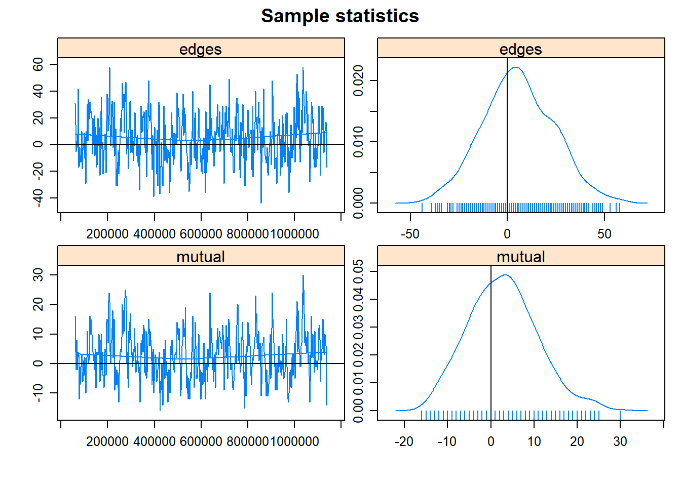
##
## MCMC diagnostics shown here are from the last round of simulation, prior to computation of final parameter estimates. Because the final estimates are refinements of those used for this simulation run, these diagnostics may understate model performance. To directly assess the performance of the final model on in-model statistics, please use the GOF command: gof(ergmFitObject, GOF=~model).
We want to see that the chains have a “fuzzy caterpillar” effect and do not have any obvious pattern to them. These chains look okay, but we might be better off if we increase the number of iterations (i.e., explore the parameter space for longer).
We can do this by adjusting the sampler controls. There are many, MANY controls for the sampler – which can be very overwhelming – so we will save those details for an advanced meeting.
fit2.1 = ergm(net ~ edges + mutual,
              control = control.ergm(MPLE.maxit = 10000))
## Starting maximum pseudolikelihood estimation (MPLE):## Evaluating the predictor and response matrix.## Maximizing the pseudolikelihood.## Finished MPLE.## Starting Monte Carlo maximum likelihood estimation (MCMLE):## Iteration 1 of at most 60:## Optimizing with step length 1.0000.## The log-likelihood improved by 0.1321.## Estimating equations are not within tolerance region.## Iteration 2 of at most 60:## Optimizing with step length 1.0000.## The log-likelihood improved by 0.0669.## Convergence test p-value: 0.2848. Not converged with 99% confidence; increasing sample size.
## Iteration 3 of at most 60:
## Optimizing with step length 1.0000.
## The log-likelihood improved by 0.0412.
## Convergence test p-value: 0.0261. Not converged with 99% confidence; increasing sample size.
## Iteration 4 of at most 60:
## Optimizing with step length 1.0000.
## The log-likelihood improved by 0.0025.
## Convergence test p-value: 0.0324. Not converged with 99% confidence; increasing sample size.
## Iteration 5 of at most 60:
## Optimizing with step length 1.0000.
## The log-likelihood improved by < 0.0001.
## Convergence test p-value: 0.0116. Not converged with 99% confidence; increasing sample size.
## Iteration 6 of at most 60:
## Optimizing with step length 1.0000.
## The log-likelihood improved by 0.0018.
## Convergence test p-value: 0.0156. Not converged with 99% confidence; increasing sample size.
## Iteration 7 of at most 60:
## Optimizing with step length 1.0000.
## The log-likelihood improved by 0.0086.
## Convergence test p-value: < 0.0001. Converged with 99% confidence.
## Finished MCMLE.
## Evaluating log-likelihood at the estimate. Fitting the dyad-independent submodel...
## Bridging between the dyad-independent submodel and the full model...
## Setting up bridge sampling...
## Using 16 bridges: 1 2 3 4 5 6 7 8 9 10 11 12 13 14 15 16 .
## Bridging finished.
## This model was fit using MCMC. To examine model diagnostics and check
## for degeneracy, use the mcmc.diagnostics() function.mcmc.diagnostics(fit2.1)## Sample statistics summary:
##
## Iterations = 114688:2240512
## Thinning interval = 4096
## Number of chains = 1
## Sample size per chain = 520
##
## 1. Empirical mean and standard deviation for each variable,
## plus standard error of the mean:
##
## Mean SD Naive SE Time-series SE
## edges -1.858 18.839 0.8261 1.0061
## mutual -1.017 7.771 0.3408 0.4747
##
## 2. Quantiles for each variable:
##
## 2.5% 25% 50% 75% 97.5%
## edges -38.02 -15 -1.5 11 36.02
## mutual -15.00 -7 -1.0 4 16.00
##
##
## Are sample statistics significantly different from observed?
## edges mutual Overall (Chi^2)
## diff. -1.85769231 -1.01730769 NA
## test stat. -1.84645780 -2.14304768 4.80323892
## P-val. 0.06482576 0.03210927 0.09262173
##
## Sample statistics cross-correlations:
## edges mutual
## edges 1.00000 0.79386
## mutual 0.79386 1.00000
##
## Sample statistics auto-correlation:
## Chain 1
## edges mutual
## Lag 0 1.000000000 1.000000000
## Lag 4096 0.279481847 0.318993211
## Lag 8192 0.079380889 0.094928989
## Lag 12288 -0.064164706 0.006576045
## Lag 16384 -0.009065296 -0.056344650
## Lag 20480 0.020932016 0.015447910
##
## Sample statistics burn-in diagnostic (Geweke):
## Chain 1
##
## Fraction in 1st window = 0.1
## Fraction in 2nd window = 0.5
##
## edges mutual
## 0.4739 0.4979
##
## Individual P-values (lower = worse):
## edges mutual
## 0.6355818 0.6185422
## Joint P-value (lower = worse): 0.937375 .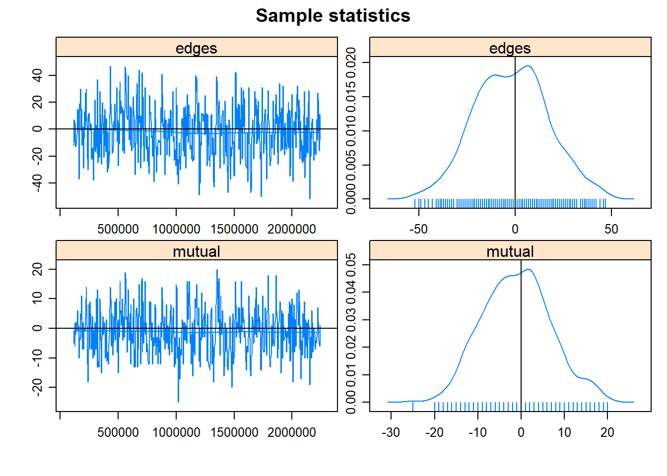
##
## MCMC diagnostics shown here are from the last round of simulation, prior to computation of final parameter estimates. Because the final estimates are refinements of those used for this simulation run, these diagnostics may understate model performance. To directly assess the performance of the final model on in-model statistics, please use the GOF command: gof(ergmFitObject, GOF=~model).
That looks a bit better. Now we can examine the ERGM summary.
summary(fit2.1)## Call:
## ergm(formula = net ~ edges + mutual, control = control.ergm(MPLE.maxit = 10000))
##
## Monte Carlo Maximum Likelihood Results:
##
## Estimate Std. Error MCMC % z value Pr(>|z|)
## edges -3.39920 0.08747 0 -38.86 <1e-04 ***
## mutual 3.43561 0.21207 0 16.20 <1e-04 ***
## ---
## Signif. codes: 0 '***' 0.001 '**' 0.01 '*' 0.05 '.' 0.1 ' ' 1
##
## Null Deviance: 6130 on 4422 degrees of freedom
## Residual Deviance: 1802 on 4420 degrees of freedom
##
## AIC: 1806 BIC: 1819 (Smaller is better. MC Std. Err. = 1.187)We see from the output that indeed, there is strong effect of reciprocity within this network. An edge from i to j is 31.05 time more likely if there exists an edge from j to i.
exp(coef(fit2.1))## edges mutual
## 0.03340002 31.05037481This leads to the question of whether reciprocity is common between households from the same family. One way to test this is by creating a new model with both nodematch and mutual. It is possible that reciprocity arrise merely because of family dynamics. If this is true, we should see a change in the coefficient estimates. If they both remain the same, or get stronger, then perhaps reciprocity and family dynamics are different independent influences on sharing.
fit2.2 = ergm(net ~ edges + nodematch('family') + mutual)## Starting maximum pseudolikelihood estimation (MPLE):## Evaluating the predictor and response matrix.## Maximizing the pseudolikelihood.## Finished MPLE.## Starting Monte Carlo maximum likelihood estimation (MCMLE):## Iteration 1 of at most 60:## Optimizing with step length 1.0000.## The log-likelihood improved by 0.0796.## Convergence test p-value: 0.6904. Not converged with 99% confidence; increasing sample size.
## Iteration 2 of at most 60:
## Optimizing with step length 1.0000.
## The log-likelihood improved by 0.0090.
## Convergence test p-value: 0.2682. Not converged with 99% confidence; increasing sample size.
## Iteration 3 of at most 60:
## Optimizing with step length 1.0000.
## The log-likelihood improved by 0.0145.
## Convergence test p-value: 0.0005. Converged with 99% confidence.
## Finished MCMLE.
## Evaluating log-likelihood at the estimate. Fitting the dyad-independent submodel...
## Bridging between the dyad-independent submodel and the full model...
## Setting up bridge sampling...
## Using 16 bridges: 1 2 3 4 5 6 7 8 9 10 11 12 13 14 15 16 .
## Bridging finished.
## This model was fit using MCMC. To examine model diagnostics and check
## for degeneracy, use the mcmc.diagnostics() function.summary(fit2.2)## Call:
## ergm(formula = net ~ edges + nodematch("family") + mutual)
##
## Monte Carlo Maximum Likelihood Results:
##
## Estimate Std. Error MCMC % z value Pr(>|z|)
## edges -4.8647 0.1927 0 -25.242 <1e-04 ***
## nodematch.family 2.9822 0.2072 0 14.393 <1e-04 ***
## mutual 2.1154 0.2241 0 9.439 <1e-04 ***
## ---
## Signif. codes: 0 '***' 0.001 '**' 0.01 '*' 0.05 '.' 0.1 ' ' 1
##
## Null Deviance: 6130 on 4422 degrees of freedom
## Residual Deviance: 1378 on 4419 degrees of freedom
##
## AIC: 1384 BIC: 1403 (Smaller is better. MC Std. Err. = 0.8788)exp(coef(fit2.2))## edges nodematch.family mutual
## 0.007714095 19.731425171 8.292992524Looking at the summary and odds-ratios (OR), we see that when both terms are included together, the strength of the mutual effect is reduced. This suggests that family homophily – kinship – is driving the reciprocity. That said, there are still some distinct reciprocity effects since the effect remains positive and significant.
GOF
Let’s take another look at the goodness-of-fit.
plot(gof(fit2.2))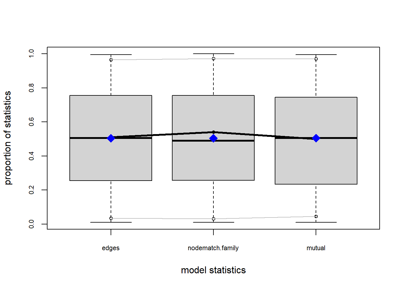
Based on these diagnostics, it seems we have improved our understanding of in-degree, but we are still missing the mark on out-degree minimum geodesic distance. Perhaps question three will help.
Question 3
In this question, we want to know understand how harvest productivity influences sharing and receiving. We might expect, for example, that individuals with large harvests are able to share with more people. We can test this with the nodeocov term.
The nodeocov term stands for node, out-degree covariance. It tests whether a nodes out-degree covaries with some vertex attribute. In our case we will use harvest. There is also a nodeicov term which tests the same thing but for in-degree.
If harvest plays a role as we expect it does, then nodeocov should be positive and nodeicov should be positive.
fit3.1 = ergm(net ~ edges + nodeocov('harvest') + nodeicov('harvest'))## Starting maximum pseudolikelihood estimation (MPLE):## Evaluating the predictor and response matrix.## Maximizing the pseudolikelihood.## Finished MPLE.## Stopping at the initial estimate.## Evaluating log-likelihood at the estimate.summary(fit3.1)## Call:
## ergm(formula = net ~ edges + nodeocov("harvest") + nodeicov("harvest"))
##
## Maximum Likelihood Results:
##
## Estimate Std. Error MCMC % z value Pr(>|z|)
## edges -3.12917 0.08802 0 -35.551 <1e-04 ***
## nodeocov.harvest 0.15280 0.03869 0 3.950 <1e-04 ***
## nodeicov.harvest 0.34740 0.04109 0 8.455 <1e-04 ***
## ---
## Signif. codes: 0 '***' 0.001 '**' 0.01 '*' 0.05 '.' 0.1 ' ' 1
##
## Null Deviance: 6130 on 4422 degrees of freedom
## Residual Deviance: 1951 on 4419 degrees of freedom
##
## AIC: 1957 BIC: 1976 (Smaller is better. MC Std. Err. = 0)The estimates show us that both out-degree and in-degree covary with harvest size, although the effects a rather small. In-degree has a stronger covariance. Since out-degree is a rather small effect, one follow up question we might ask is how owner influences out-degree. Perhaps it is harvest size, per se, that influences sharing connections, but rather who owns a boat. In many places, boats are the location of sharing events.
To examine the effect of boat ownership, we will use the term nodeofactor. This is similar to nodeocov except that it is designed for factors. For those who are familiar with dummy variables, a node factor behave similarly.
fit3.2 = ergm(net ~ edges + nodeocov('harvest') + nodeicov('harvest') + nodeofactor('owner'))## Starting maximum pseudolikelihood estimation (MPLE):## Evaluating the predictor and response matrix.## Maximizing the pseudolikelihood.## Finished MPLE.## Stopping at the initial estimate.## Evaluating log-likelihood at the estimate.summary(fit3.2)## Call:
## ergm(formula = net ~ edges + nodeocov("harvest") + nodeicov("harvest") +
## nodeofactor("owner"))
##
## Maximum Likelihood Results:
##
## Estimate Std. Error MCMC % z value Pr(>|z|)
## edges -3.26609 0.09477 0 -34.463 < 1e-04 ***
## nodeocov.harvest 0.10709 0.04139 0 2.587 0.00968 **
## nodeicov.harvest 0.34981 0.04131 0 8.467 < 1e-04 ***
## nodeofactor.owner.1 0.74291 0.14691 0 5.057 < 1e-04 ***
## ---
## Signif. codes: 0 '***' 0.001 '**' 0.01 '*' 0.05 '.' 0.1 ' ' 1
##
## Null Deviance: 6130 on 4422 degrees of freedom
## Residual Deviance: 1927 on 4418 degrees of freedom
##
## AIC: 1935 BIC: 1961 (Smaller is better. MC Std. Err. = 0)When we include ownership, we find that the effect of harvest size is diminished and becomes less signifcant, while boat ownership itself is a much stronger effect.
Even so, it seems that households with large harvest still tend to share more often, even if they don’t have a boat. We can test this explicitly. What is the probably of edge if a household has a large harvest but no boat vs. the same household with a boat?
To do this, I am saving the log-odds coefficients, then I plug them into the logit2prob function and multiply them by the harvest size and boat ownership values. Here I am compare harvest of size 4, which is about 4,000 lbs.
coef3.2 = coef(fit3.2)

# no boat
logit2prob( coef3.2[1] + coef3.2[2]*4 + coef3.2[4]*0 )
## edges
## 0.05531871logit2prob( coef3.2[1] + coef3.2[2]*4 + coef3.2[4]*1 )## edges
## 0.1096008Combined models
We have three conclusions so far:
- Kinship and family groups have a strong positive influence on sharing relationships.
- Reciprocity also has a strong positive effect, although it is partly driven by kinship and partly driven by reciprocity between non-kin.
- Owning a boat is assocated with more sharing connections, while having a small harvest is assocaited with being on the receiving end of more partnerships.
Let’s combine each of these hypotheses into a single model and see if there are any obvious changes to these conclusions. The main reason for doing this is so that we can determine the relative strengths of each effect against the others.
fit4.1 = ergm(net ~ edges + nodematch('family') + mutual + nodeocov('harvest') + nodeicov('harvest') + nodeofactor('owner'))## Starting maximum pseudolikelihood estimation (MPLE):## Evaluating the predictor and response matrix.## Maximizing the pseudolikelihood.## Finished MPLE.## Starting Monte Carlo maximum likelihood estimation (MCMLE):## Iteration 1 of at most 60:## Optimizing with step length 1.0000.## The log-likelihood improved by 0.3656.## Estimating equations are not within tolerance region.## Iteration 2 of at most 60:## Optimizing with step length 1.0000.## The log-likelihood improved by 0.0541.## Convergence test p-value: 0.2372. Not converged with 99% confidence; increasing sample size.
## Iteration 3 of at most 60:
## Optimizing with step length 1.0000.
## The log-likelihood improved by 0.0639.
## Convergence test p-value: 0.5243. Not converged with 99% confidence; increasing sample size.
## Iteration 4 of at most 60:
## Optimizing with step length 1.0000.
## The log-likelihood improved by 0.0553.
## Convergence test p-value: 0.2400. Not converged with 99% confidence; increasing sample size.
## Iteration 5 of at most 60:
## Optimizing with step length 1.0000.
## The log-likelihood improved by 0.1144.
## Estimating equations are not within tolerance region.
## Estimating equations did not move closer to tolerance region more than 1 time(s) in 4 steps; increasing sample size.
## Iteration 6 of at most 60:
## Optimizing with step length 1.0000.
## The log-likelihood improved by 0.0939.
## Convergence test p-value: 0.0002. Converged with 99% confidence.
## Finished MCMLE.
## Evaluating log-likelihood at the estimate. Fitting the dyad-independent submodel...
## Bridging between the dyad-independent submodel and the full model...
## Setting up bridge sampling...
## Using 16 bridges: 1 2 3 4 5 6 7 8 9 10 11 12 13 14 15 16 .
## Bridging finished.
## This model was fit using MCMC. To examine model diagnostics and check
## for degeneracy, use the mcmc.diagnostics() function.summary(fit4.1)## Call:
## ergm(formula = net ~ edges + nodematch("family") + mutual + nodeocov("harvest") +
## nodeicov("harvest") + nodeofactor("owner"))
##
## Monte Carlo Maximum Likelihood Results:
##
## Estimate Std. Error MCMC % z value Pr(>|z|)
## edges -5.580005 0.215826 0 -25.854 <1e-04 ***
## nodematch.family 3.177944 0.219409 0 14.484 <1e-04 ***
## mutual 2.008886 0.246330 0 8.155 <1e-04 ***
## nodeocov.harvest 0.003266 0.049497 0 0.066 0.947
## nodeicov.harvest 0.427652 0.050962 0 8.392 <1e-04 ***
## nodeofactor.owner.1 1.064196 0.186527 0 5.705 <1e-04 ***
## ---
## Signif. codes: 0 '***' 0.001 '**' 0.01 '*' 0.05 '.' 0.1 ' ' 1
##
## Null Deviance: 6130 on 4422 degrees of freedom
## Residual Deviance: 1248 on 4416 degrees of freedom
##
## AIC: 1260 BIC: 1298 (Smaller is better. MC Std. Err. = 0.7166)When all of these effects are combined, we find that many of the estimates are the same as before. One key difference is that harvest size no longer has any effect on the number of giving relationships. We also see that boat ownership is a stronger effect in the presence of family ties and reciprocity. This suggests that people may reciprocate outside of their family with people who own boats.
Goodness-of-fit
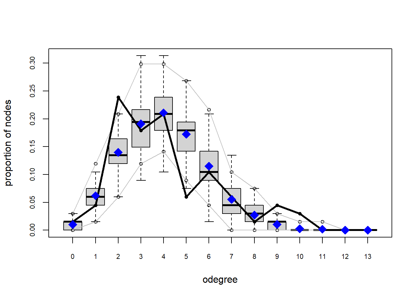
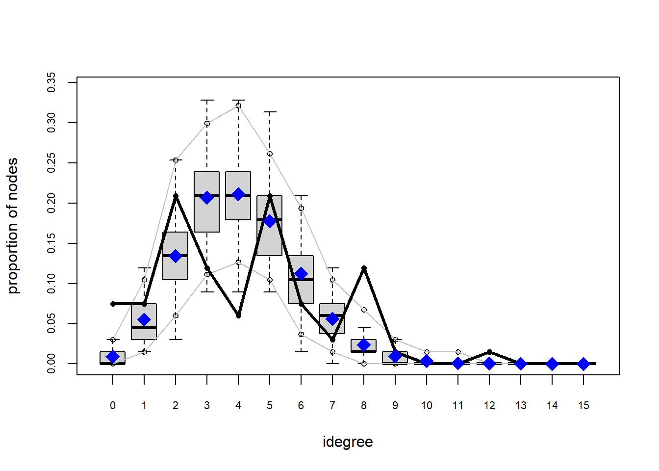
Let’s examine the gof function again and see how well we capture the observed structural values of the network. Recall that previous models had a difficult time capturing the degree distributions.
plot(gof(fit4.1))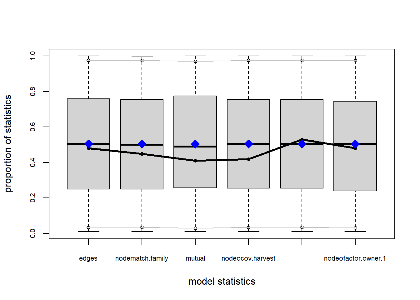
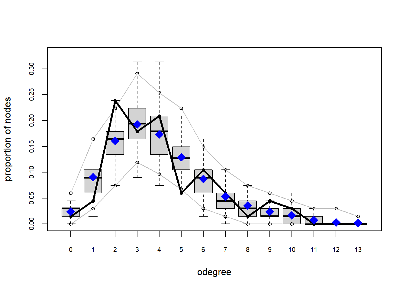
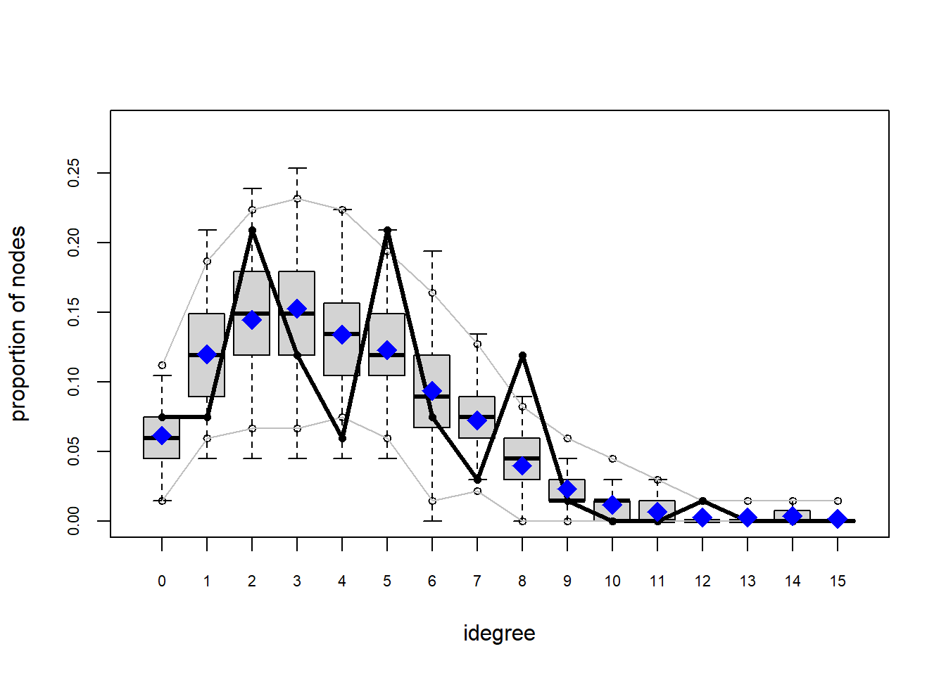
 It appears that we are still have some issues but overall there fit is reasonable. We can further fine tune this model by include some additional structural parameters.
Instead of looking at graphs, we can also use the gof hypothesis testing approach.
gof(fit4.1, GOF = ~model)##
## Goodness-of-fit for model statistics
##
## obs min mean max MC p-value
## edges 272.0000 244.0000 272.1700 310.0000 0.98
## nodematch.family 245.0000 222.0000 245.3300 280.0000 0.98
## mutual 69.0000 47.0000 69.1300 86.0000 1.00
## nodeocov.harvest 231.4796 144.0366 229.5862 281.4167 0.92
## nodeicov.harvest 358.2104 296.3139 355.3261 416.5988 0.86
## nodeofactor.owner.1 81.0000 64.0000 81.2200 96.0000 0.96The resulting table tells us statistically how well these terms fit our data. In this case, p-values closer to 1 are better. We find that of all of the terms, ownership is the worst fit, but it is still relatively high.
Bonus: triangles
Perhaps we should control for the tends for families to close triads within them. We can do this by explicit including terms for certain types of triads (e.g., cycles) or we can use the gwesp term. The gwesp term estimates the tendency for triadic closure within a network (for more details, see this workshop).
GWESP stands for geometrics weighted edgewise shared partners. This terms described the tendency for a triangle to close when two individuals have a shared partners. If the values is high, then there is a tendency for closure. It small networks, it is often the case that adding a single tie can closure several triangles.
Some analysts use gwesp as a control parameters that helps them get clearer estimates for other variables of interest. Others may be testing competing hypotheses: for example, is a network driven more by homophily or triadic closure? In our case, we want to know if closure within families leads to a more even degree distribution.
In ?ergm-terms there is also a triangles term. This estimates how much more likely a tie is based on the number of shared partners. In other words, each additional shared partner continues to additively increase the probability. In contrast, the gwesp term uses a decay parameter with discounts each additional partner, making it a more conservative estimate of triadic closure.
fit4.2 = ergm(net ~ edges + nodematch('family') + mutual + nodeocov('harvest') + nodeicov('harvest') + nodeofactor('owner') + gwesp(0.5, fixed=T))## Starting maximum pseudolikelihood estimation (MPLE):## Evaluating the predictor and response matrix.## Maximizing the pseudolikelihood.## Finished MPLE.## Starting Monte Carlo maximum likelihood estimation (MCMLE):## Iteration 1 of at most 60:## Optimizing with step length 1.0000.## The log-likelihood improved by 0.5816.## Estimating equations are not within tolerance region.## Iteration 2 of at most 60:## Optimizing with step length 1.0000.## The log-likelihood improved by 0.0595.## Convergence test p-value: 0.9105. Not converged with 99% confidence; increasing sample size.
## Iteration 3 of at most 60:
## Optimizing with step length 1.0000.
## The log-likelihood improved by 0.0558.
## Convergence test p-value: 0.7967. Not converged with 99% confidence; increasing sample size.
## Iteration 4 of at most 60:
## Optimizing with step length 1.0000.
## The log-likelihood improved by 0.1001.
## Convergence test p-value: 0.2075. Not converged with 99% confidence; increasing sample size.
## Iteration 5 of at most 60:
## Optimizing with step length 1.0000.
## The log-likelihood improved by 0.0292.
## Convergence test p-value: 0.0123. Not converged with 99% confidence; increasing sample size.
## Iteration 6 of at most 60:
## Optimizing with step length 1.0000.
## The log-likelihood improved by 0.0226.
## Convergence test p-value: 0.0370. Not converged with 99% confidence; increasing sample size.
## Iteration 7 of at most 60:
## Optimizing with step length 1.0000.
## The log-likelihood improved by 0.0258.
## Convergence test p-value: 0.0018. Converged with 99% confidence.
## Finished MCMLE.
## Evaluating log-likelihood at the estimate. Fitting the dyad-independent submodel...
## Bridging between the dyad-independent submodel and the full model...
## Setting up bridge sampling...
## Using 16 bridges: 1 2 3 4 5 6 7 8 9 10 11 12 13 14 15 16 .
## Bridging finished.
## This model was fit using MCMC. To examine model diagnostics and check
## for degeneracy, use the mcmc.diagnostics() function.summary(fit4.2)## Call:
## ergm(formula = net ~ edges + nodematch("family") + mutual + nodeocov("harvest") +
## nodeicov("harvest") + nodeofactor("owner") + gwesp(0.5, fixed = T))
##
## Monte Carlo Maximum Likelihood Results:
##
## Estimate Std. Error MCMC % z value Pr(>|z|)
## edges -5.63401 0.22765 0 -24.749 <1e-04 ***
## nodematch.family 3.34608 0.27240 0 12.284 <1e-04 ***
## mutual 2.03767 0.24065 0 8.467 <1e-04 ***
## nodeocov.harvest 0.01885 0.05437 0 0.347 0.729
## nodeicov.harvest 0.44744 0.05579 0 8.020 <1e-04 ***
## nodeofactor.owner.1 1.15738 0.19481 0 5.941 <1e-04 ***
## gwesp.fixed.0.5 -0.09793 0.08278 0 -1.183 0.237
## ---
## Signif. codes: 0 '***' 0.001 '**' 0.01 '*' 0.05 '.' 0.1 ' ' 1
##
## Null Deviance: 6130 on 4422 degrees of freedom
## Residual Deviance: 1248 on 4415 degrees of freedom
##
## AIC: 1262 BIC: 1307 (Smaller is better. MC Std. Err. = 0.9049)This estimate indicates that there are not many edges that would close triangles which suggests that there are relatively few shared partners in this network. This makes sense since the network itself is somewhat cluster into family groups. Were these groups not present, there may be a stronger triangle effect.
Model Comparison
We have many models now and each one has helped us understand a specific aspect of household sharing. We could stop there but it might also be useful to learn which model makes the strongest predictions about the network structure.
We need to be careful when we do and talk about model comparison. Every model we create is wrong. But they can be useful. Some researchers have a tendencies to describe the “best” model or the “correct” model. But these ideas only make sense in the context of prediction, we are interested in inference.
Information Criterion
One way to compare models is to use Information Criterion like AIC or BIC. We can use the AIC function to rank our model objects. This will help us learn more about what underlies the network formation. Using AIC, lower values indicate more predictive power.
mcomp = AIC(fit0, fit1.1, fit2.1, fit2.2, fit3.1, fit3.2, fit4.1, fit4.2)
mcomp[ order(mcomp$AIC), ]
## df AIC
## fit4.1 6 1259.675
## fit4.2 7 1261.968
## fit2.2 3 1383.637
## fit1.1 2 1469.528
## fit2.1 2 1805.717
## fit3.2 4 1935.423
## fit3.1 3 1957.276
## fit0 1 2045.884AIC analysis shows that the models that have our node covariates and structural parameters have the most predictive power. Notably, the model with the gwesp term is not a strong as the model without it. We also see that the models that only have node covariates (fit3.1 and fit3.2) do not have the same predictive power as the models that contain mutual.
Analysis of Deviance
Another approach we can use is to compare the deviance between the models. Every ERGM calculate a measure of Null deviance. This is reported at the bottom of each of the model summaries.
summary(fit0)## Call:
## ergm(formula = net ~ edges)
##
## Maximum Likelihood Results:
##
## Estimate Std. Error MCMC % z value Pr(>|z|)
## edges -2.72506 0.06259 0 -43.54 <1e-04 ***
## ---
## Signif. codes: 0 '***' 0.001 '**' 0.01 '*' 0.05 '.' 0.1 ' ' 1
##
## Null Deviance: 6130 on 4422 degrees of freedom
## Residual Deviance: 2044 on 4421 degrees of freedom
##
## AIC: 2046 BIC: 2052 (Smaller is better. MC Std. Err. = 0)The Null deviance is the same for every one of our models. It is a constant value derived from the network object itself. For this network, the NULL deviance is 6130. Each model then also reports the Residual deviance – the deviance that is left unexplained by the model.
summary(fit1.1)## Call:
## ergm(formula = net ~ edges + nodematch("family"))
##
## Maximum Likelihood Results:
##
## Estimate Std. Error MCMC % z value Pr(>|z|)
## edges -4.8134 0.1932 0 -24.91 <1e-04 ***
## nodematch.family 3.5993 0.2065 0 17.43 <1e-04 ***
## ---
## Signif. codes: 0 '***' 0.001 '**' 0.01 '*' 0.05 '.' 0.1 ' ' 1
##
## Null Deviance: 6130 on 4422 degrees of freedom
## Residual Deviance: 1466 on 4420 degrees of freedom
##
## AIC: 1470 BIC: 1482 (Smaller is better. MC Std. Err. = 0)So we can compare every model and see which models have the smallest residual deviance. This is an indication how much variance has been explain by the ERGM.
The ANOVA function used for this procedure will compare the model sequentially. This means that the order matters! This means that each of our eight models needs to be compared pairwise to each of the other models. For our purposes, we are only going to compare the top three models.
anova(fit4.1, fit4.2)## Analysis of Variance Table
##
## Model 1: net ~ edges + nodematch("family") + mutual + nodeocov("harvest") +
## nodeicov("harvest") + nodeofactor("owner")
## Model 2: net ~ edges + nodematch("family") + mutual + nodeocov("harvest") +
## nodeicov("harvest") + nodeofactor("owner") + gwesp(0.5, fixed = T)
## Df Deviance Resid. Df Resid. Dev Pr(>|Chisq|)
## NULL 4422 6130.2
## 1 6 4882.5 4416 1247.7 <2e-16 ***
## 2 1 -0.3 4415 1248.0 0.5882
## ---
## Signif. codes: 0 '***' 0.001 '**' 0.01 '*' 0.05 '.' 0.1 ' ' 1anova(fit4.1, fit2.2)## Analysis of Variance Table
##
## Model 1: net ~ edges + nodematch("family") + mutual + nodeocov("harvest") +
## nodeicov("harvest") + nodeofactor("owner")
## Model 2: net ~ edges + nodematch("family") + mutual
## Df Deviance Resid. Df Resid. Dev Pr(>|Chisq|)
## NULL 4422 6130.2
## 1 6 4882.5 4416 1247.7 < 2.2e-16 ***
## 2 -3 -130.0 4419 1377.6 < 2.2e-16 ***
## ---
## Signif. codes: 0 '***' 0.001 '**' 0.01 '*' 0.05 '.' 0.1 ' ' 1anova(fit2.2, fit4.2)## Analysis of Variance Table
##
## Model 1: net ~ edges + nodematch("family") + mutual
## Model 2: net ~ edges + nodematch("family") + mutual + nodeocov("harvest") +
## nodeicov("harvest") + nodeofactor("owner") + gwesp(0.5, fixed = T)
## Df Deviance Resid. Df Resid. Dev Pr(>|Chisq|)
## NULL 4422 6130.2
## 1 3 4752.6 4419 1377.6 < 2.2e-16 ***
## 2 4 129.7 4415 1248.0 < 2.2e-16 ***
## ---
## Signif. codes: 0 '***' 0.001 '**' 0.01 '*' 0.05 '.' 0.1 ' ' 1These results tell us that fit4.1 and fit4.2 are nearly identical. Their residual deviance only differs by -0.3. The p-value also shows they are not significantly different from each other. However, both 4.1 and 4.2 clearly outperform fit2.2.
We can take these comparisons as evidence that there is both household level attributes (harvest size) and dyadic attributes (kinship and reciprocity) that are needed to describe the structure of this network.
Conclusions
In conclusion, I want to let you all in on a little secret… This is not a real dataset. I SIMULATED IT. Although I based my simulation based on previous work that I have done on food sharing in Alaska (Scaggs et al. 2021), the network we analyzed here was synthetically generated using an ERGM model. The code for this is shown below:
set.seed(777)
N = 67
net = network(N, density=0)
net %v% 'owner'   = sample(c(0,1), size=N, prob = c(0.8,0.2), replace = T)
net %v% 'family'  = sample(LETTERS[1:4], size=N, prob = c(0.2,0.25,0.25,0.3), replace = T)
net %v% 'harvest' = ifelse( net %v% 'owner' == 1, rnorm(N, 2,1), rnorm(N,0,2))
net %v% 'hhsize'  = rnorm(N)

simnet = simulate(net ~ edges +
                      nodeofactor('owner') +
                      nodematch('family') +
                      nodeocov('harvest') +
                      nodeicov('harvest') +
                      gwesp(decay=0.1, fixed=T) +
                      mutual +
                      isolates,
                  coef = c(-6,       # density
                            1.5,     # ownership effect
                            3.5,     # family homophily
                            0,       # large harvest giving
                            0.5,     # small harvest receiving
                            0,       # shared partnerships
                            2,       # reciprocity
                           -2),      # isolates
                  seed = 777)

saveRDS(simnet, file = 'fishing_network.Rdata')
I did this to demonstrate two important things. First, ERGMs are generative models – they can be used to created simulated data sets similar to the way that Bayesian models can be used to generate test data.
Secondly, simulating and modeling simulated data is an important way to validate your own causal assumptions and anticipate possible confounding effects in data. In a real analysis, I would use this same procedure:
- Set some causal assumptions about how a network forms.
- Simulate multiple networks based on different causal scenarios and fit ERGM models to these networks.
- Apply developed models to empirical data and compare the results to the simulated results.
By thinking about the data generation process and conducting causal simulations, we are better able to replicate results, make our own studies reproducible, and – most importantly – make better causal inferences about the processes that occur in the systems we study.
In a future meeting, we will dig deeper into simulation, including using the results from and ERGM analysis to generate additional networks. Until then, you can also check out our posting on Network Simulation using statnet.
Additional resources:
statnethas many helpful workshops and tutorials- Standford anthropologists have put together a short course on social network analysis
- This course by Mark Hoffman has many useful resources, including a chapter on ERGMs
- A workshop by Ted Chen describes some useful ERGM extensions
We cited this paper above: Morris, M., Handcock, M. S., & Hunter, D. R. (2008). Specification of exponential-family random graph models: terms and computational aspects. Journal of statistical software, 24(4), 1548.
And this paper from Shane’s work: Scaggs, S. A., Gerkey, D., & McLaughlin, K. R. (2021). Linking subsistence harvest diversity and productivity to adaptive capacity in an Alaskan food sharing network. American Journal of Human Biology, 33(4), e23573.