In this meeting, we cover the basics of working with networks in R. By the end of the workshop, you will be acquainted with three packages – igraph, statnet, and tidygraph – and you will be able to create a network from scratch, turn it into a network object, create vertex and edge attributes, and genereate a basic visualization. Let’s get started.
R Markdown Introduction
Before we begin talking about networks, let’s first talk about the R studio environment. Most R code can be successfully run using classic .r files.
Sometimes, it makes more sense to present information and structure R code using R Markdown .rmd, which is what this type of file is.
R Markdown contains the same capabilities as classic .r files, but has the added ability to insert text (and equations!) that can be knit into a clean-appearing .html or .pdf file for presentations or write-ups. You also have the ability to hide or show chunks of code in the “knit” file. Therefore, R markdown provides a nice format for embedding R output within a research paper (such as by only including R plots within text). Or, R markdown is great to write tutorials or show coding logic, by showing R code within text.
It’s easy to add headers (use #’s).
Example Header A
Example Subheader B
Example Tertiary Header C
Then, it’s easy to embed R code “chunks”, which always follow this basic format:
a <- 1+1
a
## [1] 2Now that we’ve discussed R markdown basics, let’s talk about network data.
Data Structures
Before we dive into network objects, let’s understand the data structures that are used to represent relational data. We will focus on matrices and edgelists, as these are among the most common structures used for network data.
Adjacency matrix
Adjacency matrix: using toy data
## [1] "i" "j" "k"## i j k
## i 0 0 0
## j 0 0 0
## k 0 0 0One way to represent a network is using a square matrix where every node in the network has its own row and column. To do this, let’s create a vector of three nodes i, j, and k.
Every cell in the matrix M represents a relationship between the two nodes – these are the network edges. A value of 0 means that no edge is present. So in this matrix, there aren’t any edges. But let’s add an edge from i to j and from i to k.
M[1,2] <- 1
M[1,3] <- 1
M
## i j k
## i 0 1 1
## j 0 0 0
## k 0 0 0This is the conventional way of representing directed edges between nodes. We can represent a reciprocal edge from k to i as well. In an undirected network, this information is redundant.
M[3,1] <- 1
M
## i j k
## i 0 1 1
## j 0 0 0
## k 1 0 0Cells along the diagonal are known as loops. For example, we can set an edge from j to j along the diagonal.
M[2,2] <- 1
M["j","j"] <- 1 #Same
M
## i j k
## i 0 1 1
## j 0 1 0
## k 1 0 0You can always extract the diagonal using diag(). This is also a handy way to set the diagonal to 0 if your network does not contain loops.
diag(M) <- 0
class(M)
## [1] "matrix" "array"M## i j k
## i 0 1 1
## j 0 0 0
## k 1 0 0Adjacency matrix: using simulated data (bernoulli)
In our example matrix above there were 3 nodes and a matrix with 9 possible edges. These means that for \(N\) nodes, there are \(N^2\) possible edges. We can use this information to simulate a random network.
set.seed(777)
# How many nodes?
N <- 7

# How many edges?
N_edges <- N^2

# Use bernoulli distribution (i.e., rbinom(size=1)) to simulate edges (coin flip)
simM <- matrix(rbinom(N_edges,
                   size=1,
                   prob=0.5),
            nrow = N)
# No loops
diag(simM) <- 0
simM
## [,1] [,2] [,3] [,4] [,5] [,6] [,7]
## [1,] 0 0 1 1 1 0 1
## [2,] 0 0 0 1 1 1 0
## [3,] 0 0 0 0 1 0 0
## [4,] 1 1 1 0 1 1 1
## [5,] 1 1 0 1 0 1 1
## [6,] 0 1 0 0 0 0 1
## [7,] 0 1 0 1 0 0 0Adjacency matrix: using real data
Let’s take a look at a sample data-set of 19 environmental issues, and their connections to each other - let’s check what this looks like in excel.
First, let’s set our working directory so that R knows where to find our file, and where to save output to.
issuenet <- read.csv("IssueIssue_Data.csv", header=T)
class(issuenet)
## [1] "data.frame"Now, let’s inspect the data as it is, and ensure it’s a matrix.
dim(issuenet) #19 rows, 19 columns! A square.## [1] 19 19class(issuenet)## [1] "data.frame"issuenet <- as.matrix(issuenet)
head(issuenet)## ï..AirQuality Forests GreenInfrast HabitatLoss Health Invasives LandUse
## [1,] NA 0.500 0.216 0.433 0.950 0.167 0.475
## [2,] 0.650 NA 0.183 0.783 0.850 0.700 0.467
## [3,] 0.400 0.233 NA 0.483 0.767 0.400 0.350
## [4,] 0.633 0.908 0.375 NA 0.767 0.833 0.425
## [5,] 0.233 0.217 0.142 0.183 NA 0.050 0.383
## [6,] 0.133 0.950 0.467 0.883 0.383 NA 0.483
## Nutrients Pests.Path Recreation RestorNatSyst RisingTemps SoilErosion
## [1,] 0.166 0.400 0.533 0.150 0.600 0.200
## [2,] 0.650 0.750 0.950 0.583 0.550 0.808
## [3,] 0.642 0.267 0.658 0.467 0.258 0.692
## [4,] 0.483 0.325 0.933 0.717 0.342 0.750
## [5,] 0.092 0.233 0.625 0.200 0.167 0.150
## [6,] 0.550 0.842 0.883 0.817 0.117 0.575
## StormWater Transportation TreeManagement VulnerableComms WarmSeason
## [1,] 0.133 0.383 0.375 0.816 0.250
## [2,] 0.817 0.300 0.367 0.417 0.675
## [3,] 0.892 0.517 0.692 0.533 0.408
## [4,] 0.700 0.300 0.500 0.583 0.425
## [5,] 0.133 0.492 0.208 0.500 0.183
## [6,] 0.667 0.475 0.733 0.300 0.283
## WaterQuality
## [1,] 0.316
## [2,] 0.850
## [3,] 0.825
## [4,] 0.717
## [5,] 0.267
## [6,] 0.617tail(issuenet)## ï..AirQuality Forests GreenInfrast HabitatLoss Health Invasives LandUse
## [14,] 0.117 0.650 0.792 0.667 0.817 0.733 0.633
## [15,] 0.950 0.583 0.533 0.800 0.792 0.700 0.917
## [16,] 0.650 0.542 0.742 0.800 0.900 0.933 0.583
## [17,] 0.267 0.467 0.192 0.350 0.867 0.350 0.342
## [18,] 0.700 0.833 0.692 0.817 0.900 0.825 0.675
## [19,] 0.083 0.217 0.358 0.758 1.000 0.567 0.517
## Nutrients Pests.Path Recreation RestorNatSyst RisingTemps SoilErosion
## [14,] 0.792 0.425 0.733 0.600 0.100 0.975
## [15,] 0.258 0.600 0.583 0.583 0.642 0.600
## [16,] 0.367 0.817 0.883 0.667 0.558 0.658
## [17,] 0.517 0.433 0.250 0.383 0.150 0.483
## [18,] 0.842 0.950 0.850 0.525 0.633 0.867
## [19,] 0.483 0.550 0.600 0.600 0.017 0.300
## StormWater Transportation TreeManagement VulnerableComms WarmSeason
## [14,] NA 0.592 0.733 0.750 0.133
## [15,] 0.742 NA 0.692 0.750 0.633
## [16,] 0.833 0.400 NA 0.758 0.542
## [17,] 0.500 0.483 0.575 NA 0.233
## [18,] 0.833 0.658 0.867 0.883 NA
## [19,] 0.300 0.233 0.000 0.783 0.050
## WaterQuality
## [14,] 0.933
## [15,] 0.642
## [16,] 0.767
## [17,] 0.467
## [18,] 0.867
## [19,] NAThere aren’t row names, currently. Let’s fix that.
rownames(issuenet) <- colnames(issuenet) #Add row names
head(issuenet)
## ï..AirQuality Forests GreenInfrast HabitatLoss Health Invasives
## ï..AirQuality NA 0.500 0.216 0.433 0.950 0.167
## Forests 0.650 NA 0.183 0.783 0.850 0.700
## GreenInfrast 0.400 0.233 NA 0.483 0.767 0.400
## HabitatLoss 0.633 0.908 0.375 NA 0.767 0.833
## Health 0.233 0.217 0.142 0.183 NA 0.050
## Invasives 0.133 0.950 0.467 0.883 0.383 NA
## LandUse Nutrients Pests.Path Recreation RestorNatSyst RisingTemps
## ï..AirQuality 0.475 0.166 0.400 0.533 0.150 0.600
## Forests 0.467 0.650 0.750 0.950 0.583 0.550
## GreenInfrast 0.350 0.642 0.267 0.658 0.467 0.258
## HabitatLoss 0.425 0.483 0.325 0.933 0.717 0.342
## Health 0.383 0.092 0.233 0.625 0.200 0.167
## Invasives 0.483 0.550 0.842 0.883 0.817 0.117
## SoilErosion StormWater Transportation TreeManagement
## ï..AirQuality 0.200 0.133 0.383 0.375
## Forests 0.808 0.817 0.300 0.367
## GreenInfrast 0.692 0.892 0.517 0.692
## HabitatLoss 0.750 0.700 0.300 0.500
## Health 0.150 0.133 0.492 0.208
## Invasives 0.575 0.667 0.475 0.733
## VulnerableComms WarmSeason WaterQuality
## ï..AirQuality 0.816 0.250 0.316
## Forests 0.417 0.675 0.850
## GreenInfrast 0.533 0.408 0.825
## HabitatLoss 0.583 0.425 0.717
## Health 0.500 0.183 0.267
## Invasives 0.300 0.283 0.617Let’s now add an “i_” to the beginning of each of our issue nodes. This will help us differentiate issue nodes from other node types later on.
colnames(issuenet) <- rownames(issuenet) <- paste0("i_", colnames(issuenet))
head(issuenet)
## i_ï..AirQuality i_Forests i_GreenInfrast i_HabitatLoss i_Health
## i_ï..AirQuality NA 0.500 0.216 0.433 0.950
## i_Forests 0.650 NA 0.183 0.783 0.850
## i_GreenInfrast 0.400 0.233 NA 0.483 0.767
## i_HabitatLoss 0.633 0.908 0.375 NA 0.767
## i_Health 0.233 0.217 0.142 0.183 NA
## i_Invasives 0.133 0.950 0.467 0.883 0.383
## i_Invasives i_LandUse i_Nutrients i_Pests.Path i_Recreation
## i_ï..AirQuality 0.167 0.475 0.166 0.400 0.533
## i_Forests 0.700 0.467 0.650 0.750 0.950
## i_GreenInfrast 0.400 0.350 0.642 0.267 0.658
## i_HabitatLoss 0.833 0.425 0.483 0.325 0.933
## i_Health 0.050 0.383 0.092 0.233 0.625
## i_Invasives NA 0.483 0.550 0.842 0.883
## i_RestorNatSyst i_RisingTemps i_SoilErosion i_StormWater
## i_ï..AirQuality 0.150 0.600 0.200 0.133
## i_Forests 0.583 0.550 0.808 0.817
## i_GreenInfrast 0.467 0.258 0.692 0.892
## i_HabitatLoss 0.717 0.342 0.750 0.700
## i_Health 0.200 0.167 0.150 0.133
## i_Invasives 0.817 0.117 0.575 0.667
## i_Transportation i_TreeManagement i_VulnerableComms
## i_ï..AirQuality 0.383 0.375 0.816
## i_Forests 0.300 0.367 0.417
## i_GreenInfrast 0.517 0.692 0.533
## i_HabitatLoss 0.300 0.500 0.583
## i_Health 0.492 0.208 0.500
## i_Invasives 0.475 0.733 0.300
## i_WarmSeason i_WaterQuality
## i_ï..AirQuality 0.250 0.316
## i_Forests 0.675 0.850
## i_GreenInfrast 0.408 0.825
## i_HabitatLoss 0.425 0.717
## i_Health 0.183 0.267
## i_Invasives 0.283 0.617Now let’s make sure that the diagonal values aren’t NA.
diag(issuenet) <- 0
issuenet
## i_ï..AirQuality i_Forests i_GreenInfrast i_HabitatLoss
## i_ï..AirQuality 0.000 0.500 0.216 0.433
## i_Forests 0.650 0.000 0.183 0.783
## i_GreenInfrast 0.400 0.233 0.000 0.483
## i_HabitatLoss 0.633 0.908 0.375 0.000
## i_Health 0.233 0.217 0.142 0.183
## i_Invasives 0.133 0.950 0.467 0.883
## i_LandUse 0.650 0.900 0.475 0.925
## i_Nutrients 0.217 0.358 0.483 0.590
## i_Pests.Path 0.250 0.883 0.267 0.883
## i_Recreation 0.733 0.850 0.458 0.833
## i_RestorNatSyst 0.325 0.683 0.617 0.750
## i_RisingTemps 0.583 0.650 0.325 0.633
## i_SoilErosion 0.675 0.625 0.608 0.650
## i_StormWater 0.117 0.650 0.792 0.667
## i_Transportation 0.950 0.583 0.533 0.800
## i_TreeManagement 0.650 0.542 0.742 0.800
## i_VulnerableComms 0.267 0.467 0.192 0.350
## i_WarmSeason 0.700 0.833 0.692 0.817
## i_WaterQuality 0.083 0.217 0.358 0.758
## i_Health i_Invasives i_LandUse i_Nutrients i_Pests.Path
## i_ï..AirQuality 0.950 0.167 0.475 0.166 0.400
## i_Forests 0.850 0.700 0.467 0.650 0.750
## i_GreenInfrast 0.767 0.400 0.350 0.642 0.267
## i_HabitatLoss 0.767 0.833 0.425 0.483 0.325
## i_Health 0.000 0.050 0.383 0.092 0.233
## i_Invasives 0.383 0.000 0.483 0.550 0.842
## i_LandUse 0.750 0.808 0.000 0.667 0.583
## i_Nutrients 0.783 0.450 0.450 0.000 0.458
## i_Pests.Path 0.833 0.658 0.483 0.427 0.000
## i_Recreation 0.867 0.808 0.725 0.542 0.767
## i_RestorNatSyst 0.708 0.817 0.842 0.600 0.750
## i_RisingTemps 0.700 0.650 0.350 0.490 0.800
## i_SoilErosion 0.583 0.783 0.592 0.825 0.425
## i_StormWater 0.817 0.733 0.633 0.792 0.425
## i_Transportation 0.792 0.700 0.917 0.258 0.600
## i_TreeManagement 0.900 0.933 0.583 0.367 0.817
## i_VulnerableComms 0.867 0.350 0.342 0.517 0.433
## i_WarmSeason 0.900 0.825 0.675 0.842 0.950
## i_WaterQuality 1.000 0.567 0.517 0.483 0.550
## i_Recreation i_RestorNatSyst i_RisingTemps i_SoilErosion
## i_ï..AirQuality 0.533 0.150 0.600 0.200
## i_Forests 0.950 0.583 0.550 0.808
## i_GreenInfrast 0.658 0.467 0.258 0.692
## i_HabitatLoss 0.933 0.717 0.342 0.750
## i_Health 0.625 0.200 0.167 0.150
## i_Invasives 0.883 0.817 0.117 0.575
## i_LandUse 0.767 0.683 0.533 0.867
## i_Nutrients 0.658 0.533 0.210 0.667
## i_Pests.Path 0.817 0.567 0.300 0.342
## i_Recreation 0.000 0.800 0.267 0.683
## i_RestorNatSyst 0.683 0.000 0.342 0.792
## i_RisingTemps 0.508 0.300 0.000 0.333
## i_SoilErosion 0.533 0.567 0.258 0.000
## i_StormWater 0.733 0.600 0.100 0.975
## i_Transportation 0.583 0.583 0.642 0.600
## i_TreeManagement 0.883 0.667 0.558 0.658
## i_VulnerableComms 0.250 0.383 0.150 0.483
## i_WarmSeason 0.850 0.525 0.633 0.867
## i_WaterQuality 0.600 0.600 0.017 0.300
## i_StormWater i_Transportation i_TreeManagement
## i_ï..AirQuality 0.133 0.383 0.375
## i_Forests 0.817 0.300 0.367
## i_GreenInfrast 0.892 0.517 0.692
## i_HabitatLoss 0.700 0.300 0.500
## i_Health 0.133 0.492 0.208
## i_Invasives 0.667 0.475 0.733
## i_LandUse 0.917 0.867 0.800
## i_Nutrients 0.533 0.217 0.400
## i_Pests.Path 0.275 0.317 0.933
## i_Recreation 0.850 0.542 0.883
## i_RestorNatSyst 0.833 0.350 0.733
## i_RisingTemps 0.583 0.217 0.683
## i_SoilErosion 0.908 0.542 0.567
## i_StormWater 0.000 0.592 0.733
## i_Transportation 0.742 0.000 0.692
## i_TreeManagement 0.833 0.400 0.000
## i_VulnerableComms 0.500 0.483 0.575
## i_WarmSeason 0.833 0.658 0.867
## i_WaterQuality 0.300 0.233 0.000
## i_VulnerableComms i_WarmSeason i_WaterQuality
## i_ï..AirQuality 0.816 0.250 0.316
## i_Forests 0.417 0.675 0.850
## i_GreenInfrast 0.533 0.408 0.825
## i_HabitatLoss 0.583 0.425 0.717
## i_Health 0.500 0.183 0.267
## i_Invasives 0.300 0.283 0.617
## i_LandUse 0.783 0.500 0.933
## i_Nutrients 0.675 0.250 0.950
## i_Pests.Path 0.717 0.083 0.750
## i_Recreation 0.617 0.383 0.833
## i_RestorNatSyst 0.542 0.558 0.917
## i_RisingTemps 0.733 0.900 0.583
## i_SoilErosion 0.733 0.279 0.967
## i_StormWater 0.750 0.133 0.933
## i_Transportation 0.750 0.633 0.642
## i_TreeManagement 0.758 0.542 0.767
## i_VulnerableComms 0.000 0.233 0.467
## i_WarmSeason 0.883 0.000 0.867
## i_WaterQuality 0.783 0.050 0.000#View(issuenet) #Can't run View() in R markdown knit#Edgelist ## The Edgelist: Using toy data
An edgelist is a more compact way to store network data. This is because it does not include the 0s in that are shown in the matrix. Instead an edgelist only contains rows for each of the edges that are present in the network. This may seem trivial for a small network of 3 nodes, but when you work with a large network with hundreds or thousands of rows, eliminating all of those zeros is very convenient.
To construct an edgelist, stack rows on top of one another using the rbind function.
E <- rbind(c('i','k'),
           c('j','j'),
           c('k','i'))
class(E)
## [1] "matrix" "array"colnames(E) <- c('Sender','Receiver')
E## Sender Receiver
## [1,] "i" "k"
## [2,] "j" "j"
## [3,] "k" "i"class(E)## [1] "matrix" "array"You can think of the first column as a sender column. The second column is a receiver column. This is how directionality is represented in the edge list.
If you want to add edges to an edgelist, simply bind a new row to the current edgelist.
E <- rbind(E, c('i','j'))
E
## Sender Receiver
## [1,] "i" "k"
## [2,] "j" "j"
## [3,] "k" "i"
## [4,] "i" "j"Use the same bracket [] notation to index, such as here, where we delete the fourth row.
E <- E[-4,]
E
## Sender Receiver
## [1,] "i" "k"
## [2,] "j" "j"
## [3,] "k" "i"But Why?
You might be wondering… why do we need to know these details about data structure? Here are two reasons.
First, whether you collect your own network data or receive data from someone else, you’ll need to store/wrangle the data into one of these formats. When you collect your own data, you can store it in this format right away. But if you receive a network you did not collect, knowing these data structures will help you understand what you are looking at.
Second, understand data structure opens the door to simulation. Put differently, you don’t need to collect data to begin learning about and visualizing networks. You can simulate synthetic data. Here is a brief example.
Edgelist: Using simulated data (bernouli graph simulation)
We can use a similar procedure to simulate an edgelist. We just need to create a third column to simulate the edges, then filter out the zeros.
set.seed(777)
N <- letters[1:5]
#or
N <- c("a","b","c","d","e")
simE <- expand.grid(N,N)
# ?expand.grid #help on this function.
simE
## Var1 Var2
## 1 a a
## 2 b a
## 3 c a
## 4 d a
## 5 e a
## 6 a b
## 7 b b
## 8 c b
## 9 d b
## 10 e b
## 11 a c
## 12 b c
## 13 c c
## 14 d c
## 15 e c
## 16 a d
## 17 b d
## 18 c d
## 19 d d
## 20 e d
## 21 a e
## 22 b e
## 23 c e
## 24 d e
## 25 e esimE$Edge <- rbinom(nrow(simE),
size = 1,
prob = 0.5)
dim(simE)## [1] 25 3head(simE) #notice 3 columns, including presence/absence of edge## Var1 Var2 Edge
## 1 a a 1
## 2 b a 0
## 3 c a 0
## 4 d a 1
## 5 e a 1
## 6 a b 0Now, let’s make this a true Edgelist, by removing rows where there is not an edge (i.e., value == 0)
simE <- simE[!simE$Edge == 0 & !simE$Var1 == simE$Var2, 1:2] #Only include edges that have a value, and that aren't loops, only show Columns 1 and 2
head(simE)
## Var1 Var2
## 4 d a
## 5 e a
## 9 d b
## 11 a c
## 12 b c
## 14 d cEdgelist: using real data
Let’s load in an edgelist - but first, let’s check out what it looks like in Excel.
aa <- read.csv("actor-actor_edgelist.csv")
head(aa)
## send receive
## 1 OEC AGC
## 2 OEC AAO
## 3 OEC AZ
## 4 OEC Au-OH
## 5 OEC AA
## 6 OEC BSCaa$send <- paste0("a_", aa$send)
aa$receive <- paste0("a_", aa$receive)Let’s inspect the data, then fix node names, which will help with future analyses.
class(aa)## [1] "data.frame"aa <- as.matrix(aa)
dim(aa)## [1] 2670 2head(aa)## send receive
## [1,] "a_OEC" "a_AGC"
## [2,] "a_OEC" "a_AAO"
## [3,] "a_OEC" "a_AZ"
## [4,] "a_OEC" "a_Au-OH"
## [5,] "a_OEC" "a_AA"
## [6,] "a_OEC" "a_BSC"Network objects in igraph
Now we will turn these data structures into igraph network objects. First, install and load the igraph package.
First let’s create some attributes for our 3 node network. They don’t need to be fancy; just some sizes and colors.
att <- data.frame(
    name = c("i","j","k"),
    size = c(20,27,34),
    color = c('tomato',
              'cornflowerblue',
              'darkorchid')
)
att
## name size color
## 1 i 20 tomato
## 2 j 27 cornflowerblue
## 3 k 34 darkorchidMatrix conversion to network
To create a network object using a matrix, we use the graph.adjacency function. In graph theory, relational matrices are often referred to as adjacency matrices. Use the M matrix that we created before.
M## i j k
## i 0 1 1
## j 0 0 0
## k 1 0 0class(M)## [1] "matrix" "array"gM <- graph.adjacency(M)
class(gM)## [1] "igraph"gM## IGRAPH b9a7dd1 DN-- 3 3 --
## + attr: name (v/c)
## + edges from b9a7dd1 (vertex names):
## [1] i->j i->k k->iWhen we call the object, we receive a summary of the network. DN means this is a directed network with 3 nodes and 3 edges. There is just one attributes, the name of the vertices. We can tell that this is a categorical vertex attribute by the notation (v/c). The edges are listed at the bottom.
Now, let’s manually add vertex attributes to the network gM from out att data frame.
gM <- set_vertex_attr(gM, name = 'size', value = att$size)
gM <- set_vertex_attr(gM, name = 'color', value = att$color)
gM
## IGRAPH b9a7dd1 DN-- 3 3 --
## + attr: name (v/c), size (v/n), color (v/c)
## + edges from b9a7dd1 (vertex names):
## [1] i->j i->k k->iEdgelist conversion to network
To create an object using an edgelist, we use the graph.data.frame function. Using edgelists is nice because you can add the vertex attribute table in directly.
E## Sender Receiver
## [1,] "i" "k"
## [2,] "j" "j"
## [3,] "k" "i"class(E)## [1] "matrix" "array"gE <- graph.data.frame(E)
#Add in the attributes
gE <- set_vertex_attr(gM, name = 'size', value = att$size)
gE <- set_vertex_attr(gM, name = 'color', value = att$color)
#Or, with one line of code to add attributes while we make igraph object:
gE <- graph.data.frame(E, vertices = att)
gE## IGRAPH b9b8271 DN-- 3 3 --
## + attr: name (v/c), size (v/n), color (v/c)
## + edges from b9b8271 (vertex names):
## [1] i->k j->j k->iclass(gE)## [1] "igraph"Once you have an igraph network object, you can extract vertex and edge attributes.
V(gE)$color## [1] "tomato" "cornflowerblue" "darkorchid"V(gE)$size## [1] 20 27 34We don’t have any edge attributes in this network, but if we did, we would use E(object)$attr syntax.
Visualize igraph objects
There are many aesthetic properties of network graph. But you can generally think of them as vertex (or node) aesthetics, edge aesthetics, and network aesthetics. To learn more about all of the ways to specify these in igraph, called ??igraph.plotting.
Let’s visualize our objects gE and gM. Here is a generic plot.
plot(gE)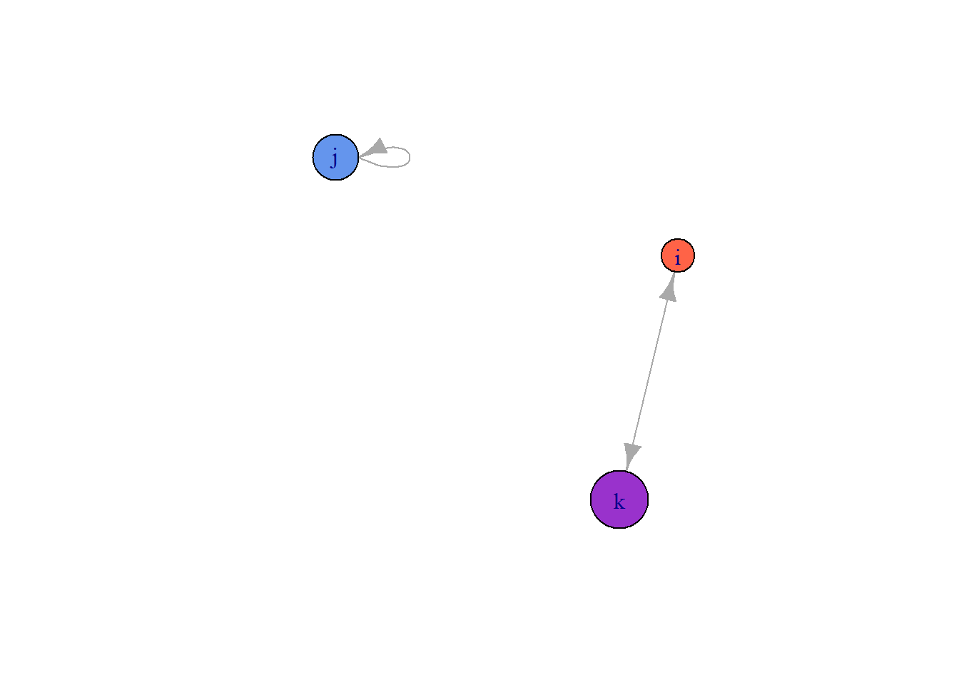
plot(gM)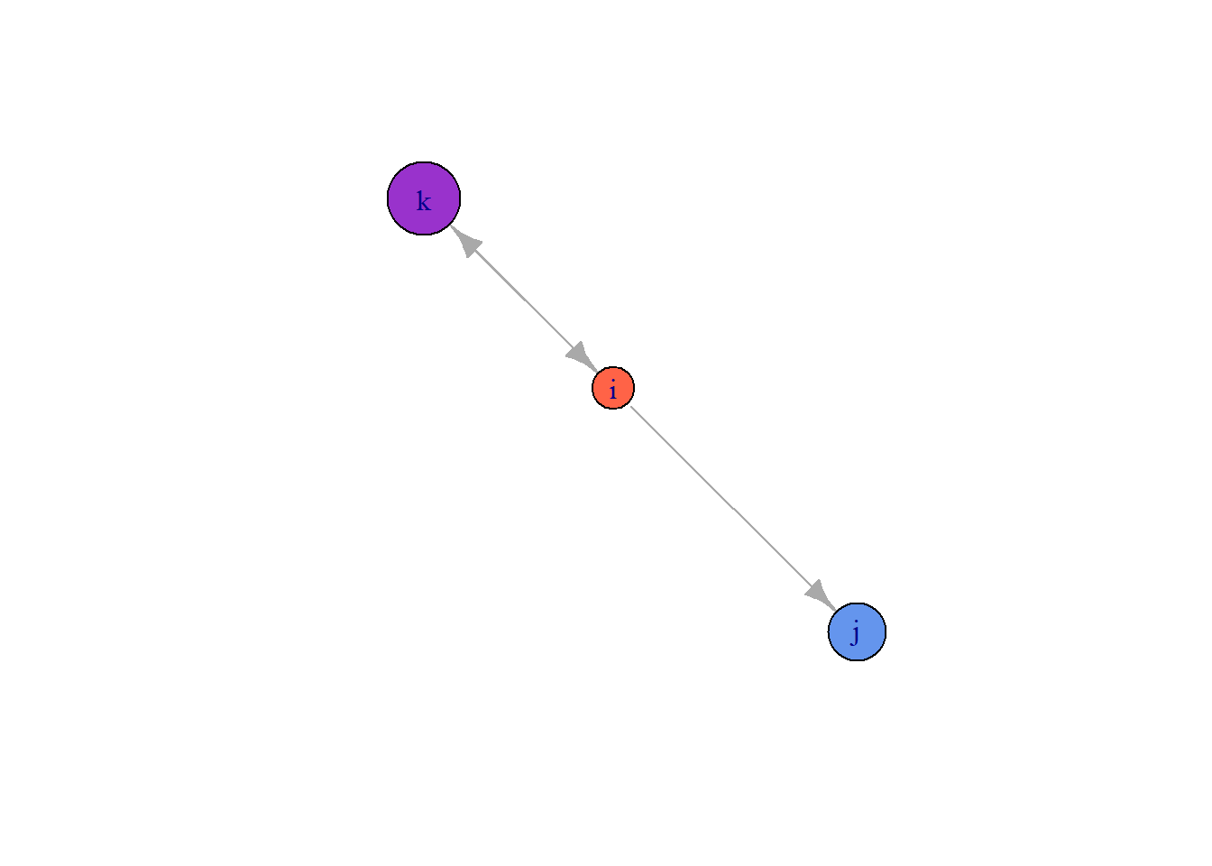
By default, igraph labels each node with the $name attribute, and, if they exist, it will choose the sizes and colors using the $color and $size attributes. Since we set size and color in our att data frame, we replaced the defaults. But we can easily override them.
plot(gE,
     vertex.color = '#2a00fa',
     vertex.size = 30)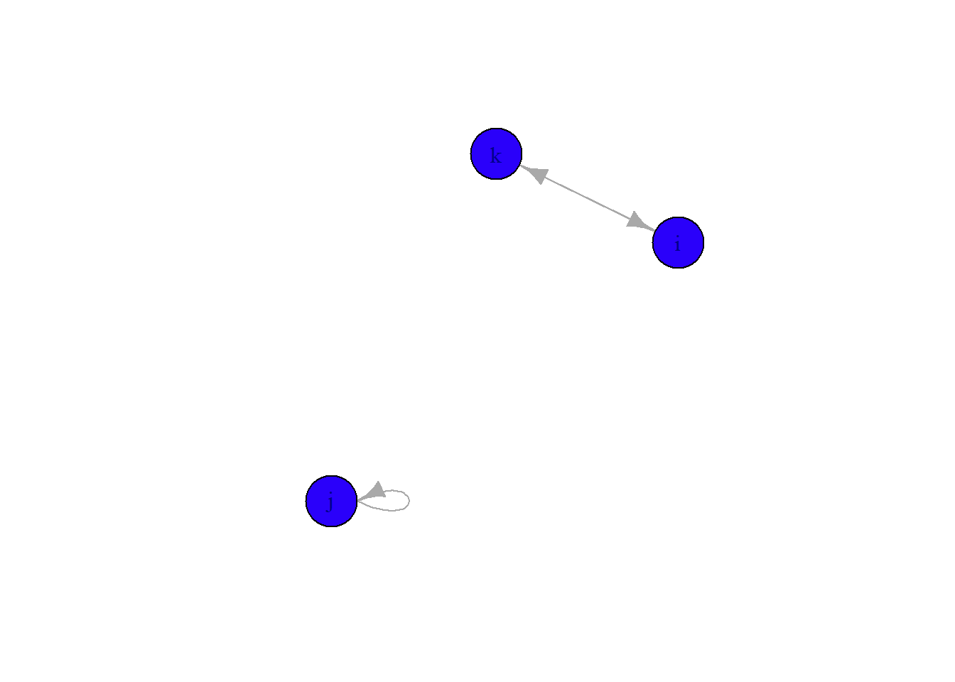
Let’s also change the color of the label to make it easier to read, change the edge colors to black, and make the arrow heads a bit smaller.
plot(gE,
     vertex.color = '#2a00fa',
     vertex.size = 30,
     vertex.label.color = 'white',
     edge.color = 'black',
     edge.arrow.size = 0.681)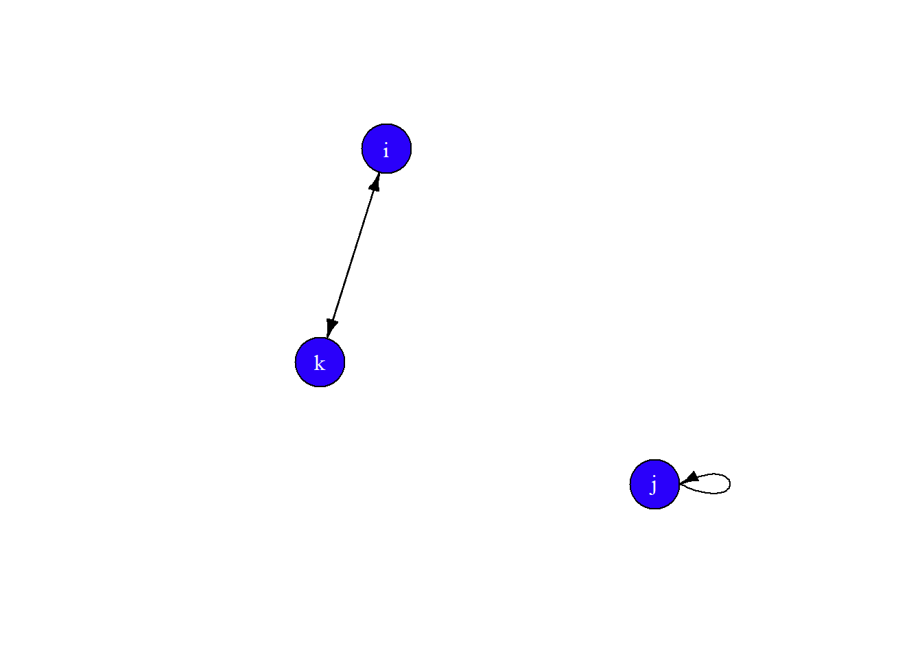
Finally, let’s set the layout to layout.circle and add some curve to the edges.
plot(gE,
     vertex.color = '#2a00fa',
     vertex.size = 30,
     vertex.label.color = 'white',
     edge.color = 'black',
     edge.arrow.size = 0.681,
     edge.curved = 0.1,
     layout = layout.circle)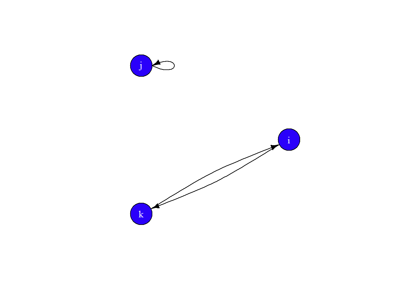
Network objects in statnet
Create network objects in statnet is pretty intuitive. First, install and load the statnet suite of packages.
To create network objects, use the network function. When using an edgelist, tell the function you are using one in the matrix.type parameter.
library(statnet)## Loading required package: tergm## Warning: package 'tergm' was built under R version 4.1.3## Loading required package: ergm## Loading required package: network##
## 'network' 1.17.1 (2021-06-12), part of the Statnet Project
## * 'news(package="network")' for changes since last version
## * 'citation("network")' for citation information
## * 'https://statnet.org' for help, support, and other information##
## Attaching package: 'network'## The following objects are masked from 'package:igraph':
##
## %c%, %s%, add.edges, add.vertices, delete.edges, delete.vertices,
## get.edge.attribute, get.edges, get.vertex.attribute, is.bipartite,
## is.directed, list.edge.attributes, list.vertex.attributes,
## set.edge.attribute, set.vertex.attribute##
## 'ergm' 4.1.2 (2021-07-26), part of the Statnet Project
## * 'news(package="ergm")' for changes since last version
## * 'citation("ergm")' for citation information
## * 'https://statnet.org' for help, support, and other information## 'ergm' 4 is a major update that introduces some backwards-incompatible
## changes. Please type 'news(package="ergm")' for a list of major
## changes.## Loading required package: networkDynamic##
## 'networkDynamic' 0.11.0 (2021-06-12), part of the Statnet Project
## * 'news(package="networkDynamic")' for changes since last version
## * 'citation("networkDynamic")' for citation information
## * 'https://statnet.org' for help, support, and other information## Registered S3 method overwritten by 'tergm':
## method from
## simulate_formula.network ergm##
## 'tergm' 4.0.2 (2021-07-28), part of the Statnet Project
## * 'news(package="tergm")' for changes since last version
## * 'citation("tergm")' for citation information
## * 'https://statnet.org' for help, support, and other information##
## Attaching package: 'tergm'## The following object is masked from 'package:ergm':
##
## snctrl## Loading required package: ergm.count##
## 'ergm.count' 4.0.2 (2021-06-18), part of the Statnet Project
## * 'news(package="ergm.count")' for changes since last version
## * 'citation("ergm.count")' for citation information
## * 'https://statnet.org' for help, support, and other information## Loading required package: sna## Loading required package: statnet.common##
## Attaching package: 'statnet.common'## The following object is masked from 'package:ergm':
##
## snctrl## The following objects are masked from 'package:base':
##
## attr, order## sna: Tools for Social Network Analysis
## Version 2.6 created on 2020-10-5.
## copyright (c) 2005, Carter T. Butts, University of California-Irvine
## For citation information, type citation("sna").
## Type help(package="sna") to get started.##
## Attaching package: 'sna'## The following objects are masked from 'package:igraph':
##
## betweenness, bonpow, closeness, components, degree, dyad.census,
## evcent, hierarchy, is.connected, neighborhood, triad.census## Loading required package: tsna## Warning: package 'tsna' was built under R version 4.1.3##
## 'statnet' 2019.6 (2019-06-13), part of the Statnet Project
## * 'news(package="statnet")' for changes since last version
## * 'citation("statnet")' for citation information
## * 'https://statnet.org' for help, support, and other information## unable to reach CRANM## i j k
## i 0 1 1
## j 0 0 0
## k 1 0 0E## Sender Receiver
## [1,] "i" "k"
## [2,] "j" "j"
## [3,] "k" "i"att## name size color
## 1 i 20 tomato
## 2 j 27 cornflowerblue
## 3 k 34 darkorchidnetM <- network(M, vertex.attr = att)
netE <- network(E, vertex.attr = att,
matrix.type = "edgelist" )
netM## Network attributes:
## vertices = 3
## directed = TRUE
## hyper = FALSE
## loops = FALSE
## multiple = FALSE
## bipartite = FALSE
## total edges= 3
## missing edges= 0
## non-missing edges= 3
##
## Vertex attribute names:
## color name size vertex.names
##
## No edge attributesnetE## Network attributes:
## vertices = 3
## directed = TRUE
## hyper = FALSE
## loops = FALSE
## multiple = FALSE
## bipartite = FALSE
## total edges= 2
## missing edges= 0
## non-missing edges= 2
##
## Vertex attribute names:
## color name size vertex.names
##
## No edge attributesc(class(netM), class(netE))## [1] "network" "network"Like the igraph object, when we call the network object, we get a summary of some important network details.
To extract variables from the network object, we use one of three operators:
%v%– extract vertex attributes%e%– extract edge attributes%n%– extract network attributes
For example, we can see the values for color by extracting the attribute from the network by calling the network object, the appropriate operator, and the name of the attribute.
netE %v% 'color'## [1] "tomato" "cornflowerblue" "darkorchid"Convert real data to igraph and network objects
igraph conversion
aa_igraph <- graph.data.frame(aa)
class(aa_igraph)
## [1] "igraph"plot(aa_igraph)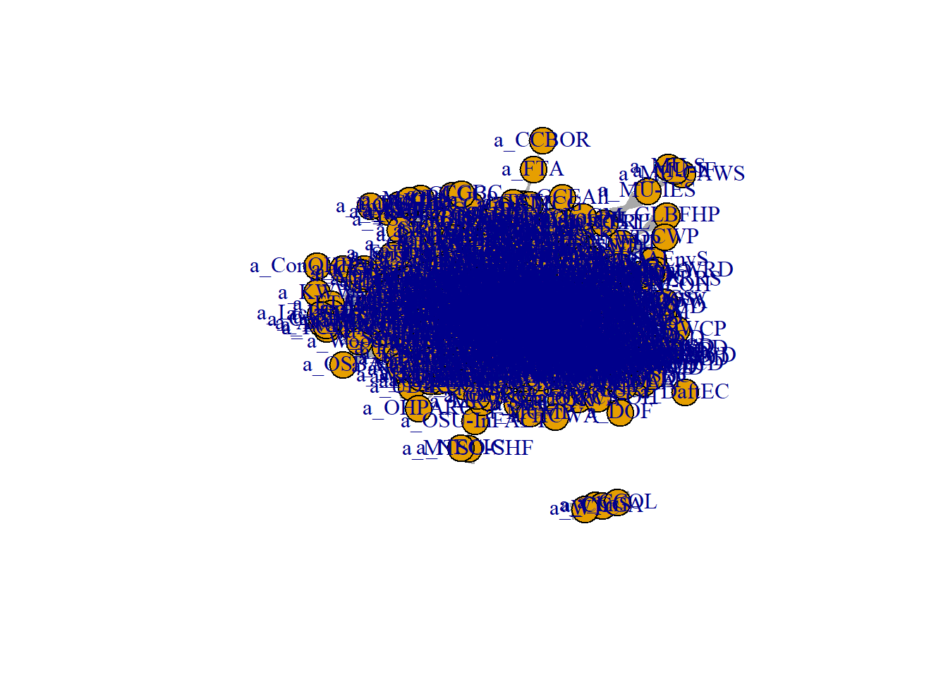
dim(aa)## [1] 2670 2Let’s plot the full network.
plot(aa_igraph)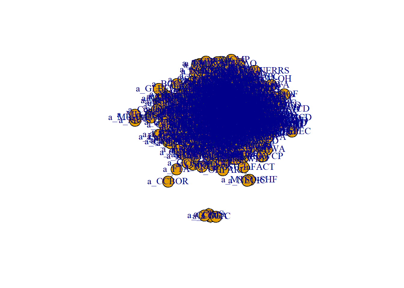
#messy!Let’s change some plot arguments to improve our graph.
plot(aa_igraph,
     vertex.color = '#2a00fa',
     vertex.size = 3,
     vertex.label = "",
     edge.color = 'black',
     edge.arrow.size = 0.02,
     edge.curved = 0.1)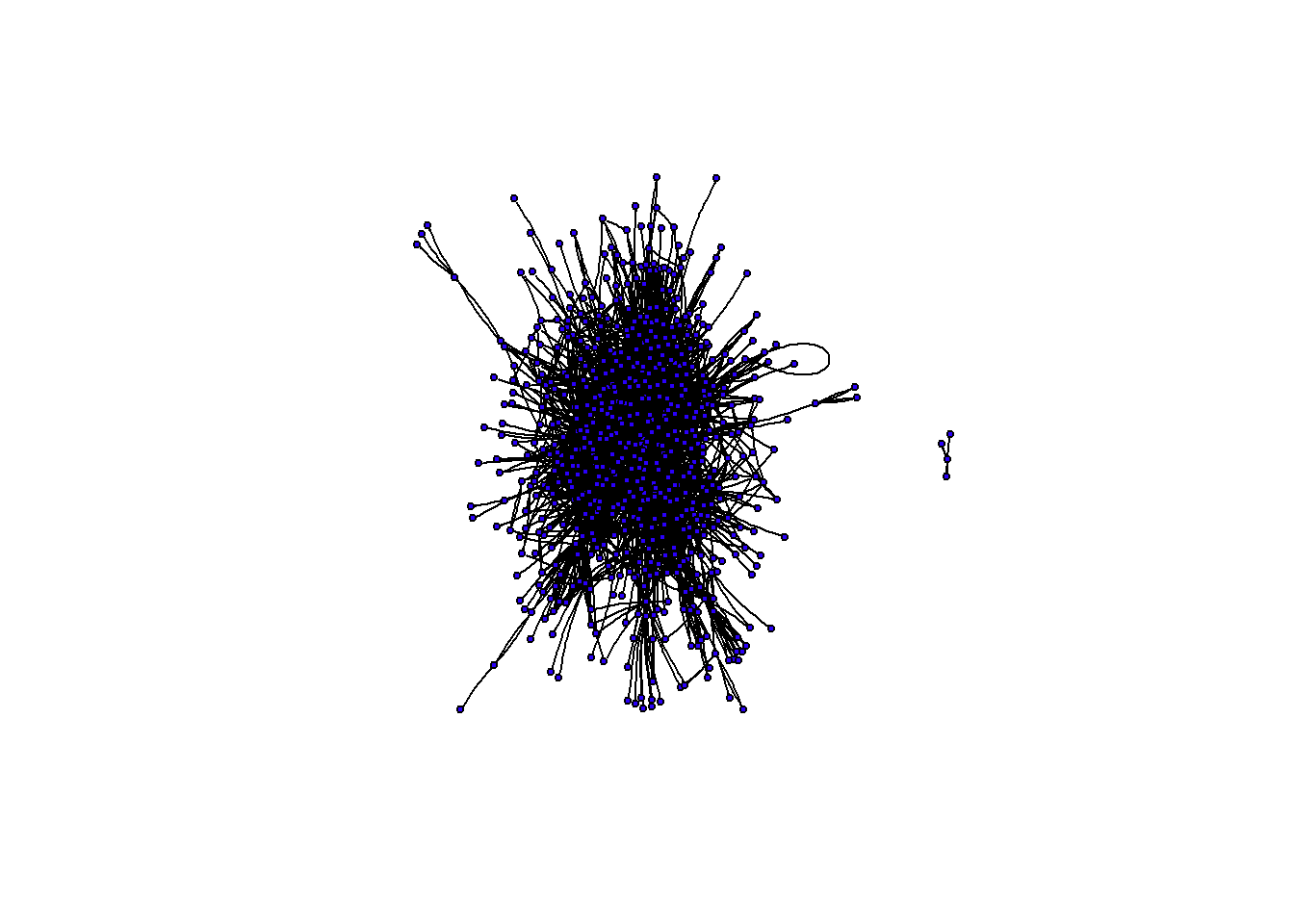
Or, we can just look at a subset of the network.
aa_shortened <- aa[1:100,]
dim(aa_shortened)
## [1] 100 2aa_igraph_shortened <- graph.data.frame(aa_shortened)Let’s plot this new, shortened network using igraph.
plot(aa_igraph_shortened,
     vertex.color = '#2a00fa',
     vertex.size = 7,
     vertex.label = "",
     edge.color = 'black',
     edge.arrow.size = 0.02,
     edge.curved = 0.1)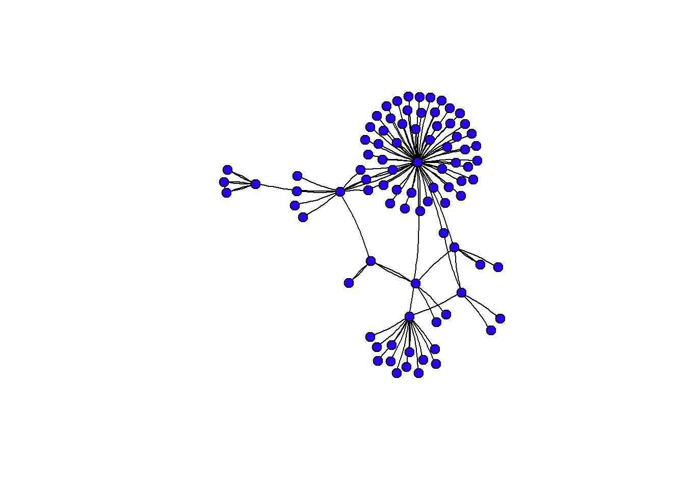
What about plotting our issue network?
issuenet## i_ï..AirQuality i_Forests i_GreenInfrast i_HabitatLoss
## i_ï..AirQuality 0.000 0.500 0.216 0.433
## i_Forests 0.650 0.000 0.183 0.783
## i_GreenInfrast 0.400 0.233 0.000 0.483
## i_HabitatLoss 0.633 0.908 0.375 0.000
## i_Health 0.233 0.217 0.142 0.183
## i_Invasives 0.133 0.950 0.467 0.883
## i_LandUse 0.650 0.900 0.475 0.925
## i_Nutrients 0.217 0.358 0.483 0.590
## i_Pests.Path 0.250 0.883 0.267 0.883
## i_Recreation 0.733 0.850 0.458 0.833
## i_RestorNatSyst 0.325 0.683 0.617 0.750
## i_RisingTemps 0.583 0.650 0.325 0.633
## i_SoilErosion 0.675 0.625 0.608 0.650
## i_StormWater 0.117 0.650 0.792 0.667
## i_Transportation 0.950 0.583 0.533 0.800
## i_TreeManagement 0.650 0.542 0.742 0.800
## i_VulnerableComms 0.267 0.467 0.192 0.350
## i_WarmSeason 0.700 0.833 0.692 0.817
## i_WaterQuality 0.083 0.217 0.358 0.758
## i_Health i_Invasives i_LandUse i_Nutrients i_Pests.Path
## i_ï..AirQuality 0.950 0.167 0.475 0.166 0.400
## i_Forests 0.850 0.700 0.467 0.650 0.750
## i_GreenInfrast 0.767 0.400 0.350 0.642 0.267
## i_HabitatLoss 0.767 0.833 0.425 0.483 0.325
## i_Health 0.000 0.050 0.383 0.092 0.233
## i_Invasives 0.383 0.000 0.483 0.550 0.842
## i_LandUse 0.750 0.808 0.000 0.667 0.583
## i_Nutrients 0.783 0.450 0.450 0.000 0.458
## i_Pests.Path 0.833 0.658 0.483 0.427 0.000
## i_Recreation 0.867 0.808 0.725 0.542 0.767
## i_RestorNatSyst 0.708 0.817 0.842 0.600 0.750
## i_RisingTemps 0.700 0.650 0.350 0.490 0.800
## i_SoilErosion 0.583 0.783 0.592 0.825 0.425
## i_StormWater 0.817 0.733 0.633 0.792 0.425
## i_Transportation 0.792 0.700 0.917 0.258 0.600
## i_TreeManagement 0.900 0.933 0.583 0.367 0.817
## i_VulnerableComms 0.867 0.350 0.342 0.517 0.433
## i_WarmSeason 0.900 0.825 0.675 0.842 0.950
## i_WaterQuality 1.000 0.567 0.517 0.483 0.550
## i_Recreation i_RestorNatSyst i_RisingTemps i_SoilErosion
## i_ï..AirQuality 0.533 0.150 0.600 0.200
## i_Forests 0.950 0.583 0.550 0.808
## i_GreenInfrast 0.658 0.467 0.258 0.692
## i_HabitatLoss 0.933 0.717 0.342 0.750
## i_Health 0.625 0.200 0.167 0.150
## i_Invasives 0.883 0.817 0.117 0.575
## i_LandUse 0.767 0.683 0.533 0.867
## i_Nutrients 0.658 0.533 0.210 0.667
## i_Pests.Path 0.817 0.567 0.300 0.342
## i_Recreation 0.000 0.800 0.267 0.683
## i_RestorNatSyst 0.683 0.000 0.342 0.792
## i_RisingTemps 0.508 0.300 0.000 0.333
## i_SoilErosion 0.533 0.567 0.258 0.000
## i_StormWater 0.733 0.600 0.100 0.975
## i_Transportation 0.583 0.583 0.642 0.600
## i_TreeManagement 0.883 0.667 0.558 0.658
## i_VulnerableComms 0.250 0.383 0.150 0.483
## i_WarmSeason 0.850 0.525 0.633 0.867
## i_WaterQuality 0.600 0.600 0.017 0.300
## i_StormWater i_Transportation i_TreeManagement
## i_ï..AirQuality 0.133 0.383 0.375
## i_Forests 0.817 0.300 0.367
## i_GreenInfrast 0.892 0.517 0.692
## i_HabitatLoss 0.700 0.300 0.500
## i_Health 0.133 0.492 0.208
## i_Invasives 0.667 0.475 0.733
## i_LandUse 0.917 0.867 0.800
## i_Nutrients 0.533 0.217 0.400
## i_Pests.Path 0.275 0.317 0.933
## i_Recreation 0.850 0.542 0.883
## i_RestorNatSyst 0.833 0.350 0.733
## i_RisingTemps 0.583 0.217 0.683
## i_SoilErosion 0.908 0.542 0.567
## i_StormWater 0.000 0.592 0.733
## i_Transportation 0.742 0.000 0.692
## i_TreeManagement 0.833 0.400 0.000
## i_VulnerableComms 0.500 0.483 0.575
## i_WarmSeason 0.833 0.658 0.867
## i_WaterQuality 0.300 0.233 0.000
## i_VulnerableComms i_WarmSeason i_WaterQuality
## i_ï..AirQuality 0.816 0.250 0.316
## i_Forests 0.417 0.675 0.850
## i_GreenInfrast 0.533 0.408 0.825
## i_HabitatLoss 0.583 0.425 0.717
## i_Health 0.500 0.183 0.267
## i_Invasives 0.300 0.283 0.617
## i_LandUse 0.783 0.500 0.933
## i_Nutrients 0.675 0.250 0.950
## i_Pests.Path 0.717 0.083 0.750
## i_Recreation 0.617 0.383 0.833
## i_RestorNatSyst 0.542 0.558 0.917
## i_RisingTemps 0.733 0.900 0.583
## i_SoilErosion 0.733 0.279 0.967
## i_StormWater 0.750 0.133 0.933
## i_Transportation 0.750 0.633 0.642
## i_TreeManagement 0.758 0.542 0.767
## i_VulnerableComms 0.000 0.233 0.467
## i_WarmSeason 0.883 0.000 0.867
## i_WaterQuality 0.783 0.050 0.000class(issuenet)## [1] "matrix" "array"gissuenet <- graph.adjacency(issuenet, weighted = T)
plot(gissuenet,
vertex.color = '#2a00fa',
vertex.size = 7,
vertex.label = "",
edge.color = 'black',
edge.arrow.size = 0.02,
edge.curved = 0.1,
edge.width=edge.betweenness(gissuenet)/10)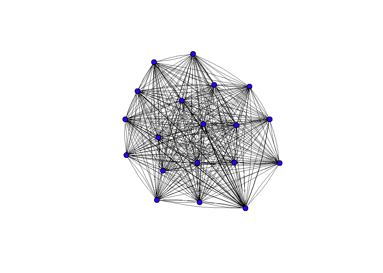
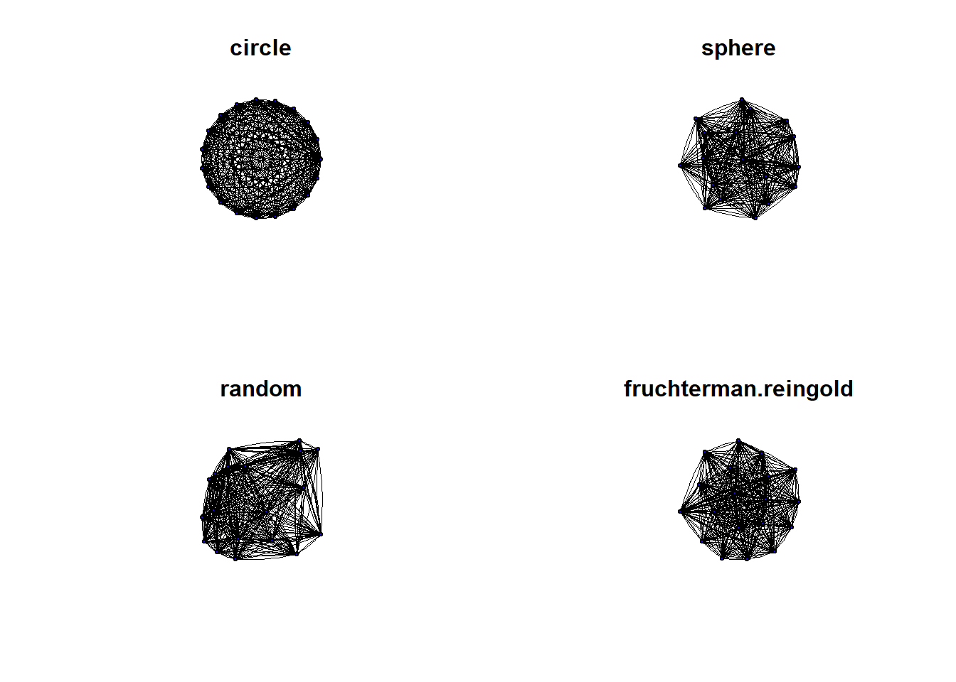
par(mfrow=c(2,2))
plota <- plot(gissuenet,
     vertex.color = '#2a00fa',
     vertex.size = 7,
     vertex.label = "",
     edge.color = 'black',
     edge.arrow.size = 0.02,
     edge.curved = 0.1,
     edge.width=edge.betweenness(gissuenet)/10,
     layout=layout.circle,
     main="circle")
plotb <- plot(gissuenet,
     vertex.color = '#2a00fa',
     vertex.size = 7,
     vertex.label = "",
     edge.color = 'black',
     edge.arrow.size = 0.02,
     edge.curved = 0.1,
     edge.width=edge.betweenness(gissuenet)/10,
     layout=layout.sphere,
     main="sphere")
plotc <- plot(gissuenet,
     vertex.color = '#2a00fa',
     vertex.size = 7,
     vertex.label = "",
     edge.color = 'black',
     edge.arrow.size = 0.02,
     edge.curved = 0.1,
     edge.width=edge.betweenness(gissuenet)/10,
     layout=layout.random,
     main="random")
plotd <- plot(gissuenet,
     vertex.color = '#2a00fa',
     vertex.size = 7,
     vertex.label = "",
     edge.color = 'black',
     edge.arrow.size = 0.02,
     edge.curved = 0.1,
     edge.width=edge.betweenness(gissuenet)/10,
     layout=layout.fruchterman.reingold,
     main="fruchterman.reingold")