A Brief Introduction to R

Panels

There are four visible panels at a time, each with different purposes (1) The R console accepts commands and produces output to your commands. (2) A text editor window to create and record code. (3) An environment window that shows your stored data in R (4) A plot/help/files window that can alternate to show your plots, help reauests, and file directory

For example, use the text editing window to write the following code:

plot(2,2)

In R Studio, notice that the code is stored in the text editor (script), is passed to the console, and then is plotted in the plot window Also, panels can be resized by dragging the slider

Getting Help

Stuck on a line of code? Not sure what a function does exactly? Want an example of someone else using that function? Use the ? before any function to pull up its help page in the Help window.

?plot

## starting httpd help server ... done

Executing Commands

Send your code from the text editor/script to the console in one of three ways: (1) Code > Run Selected Line(s) (2) Select Run Icon on top-right of Script Editor box (3) Keyboard Shortcut Mac: Command + Return Windows: Ctrl + Enter

Scripts

You can have multiple scripts in R Scripts appear as tabs in the text edit panel Save your scripts OFTEN R studio will sometimes crash unexpectedly and you could lose unsaved changes

Annotating

Have you wondered why some of the text in your script is green colored? It’s to annotate your script! Annotations are saved in the text editor window You can use them to section your script and to write notes about what your code is doing. You SHOULD annotate your script, so you can go back potentially YEARS later and still understand what you did (why did I write that code?)

Anything after the HASHTAG becomes annotated, for example:

2+2 #An easy math problem 

## [1] 4

2 #Math    + 2

## [1] 2

Notice in the second math line above, the “+2” is not added because it occurs after the #

Types of Objects

R data is stored as Objects

Common types of R Objects: Vectors: Single Dimension (a variable or column) Matrices: a data matrix Data Frames: Basically tables Data frames are COMMON and are organized like an excel worksheet. -Variables are columns -Observations are rows

mtcars

##                      mpg cyl  disp  hp drat    wt  qsec vs am gear carb
## Mazda RX4           21.0   6 160.0 110 3.90 2.620 16.46  0  1    4    4
## Mazda RX4 Wag       21.0   6 160.0 110 3.90 2.875 17.02  0  1    4    4
## Datsun 710          22.8   4 108.0  93 3.85 2.320 18.61  1  1    4    1
## Hornet 4 Drive      21.4   6 258.0 110 3.08 3.215 19.44  1  0    3    1
## Hornet Sportabout   18.7   8 360.0 175 3.15 3.440 17.02  0  0    3    2
## Valiant             18.1   6 225.0 105 2.76 3.460 20.22  1  0    3    1
## Duster 360          14.3   8 360.0 245 3.21 3.570 15.84  0  0    3    4
## Merc 240D           24.4   4 146.7  62 3.69 3.190 20.00  1  0    4    2
## Merc 230            22.8   4 140.8  95 3.92 3.150 22.90  1  0    4    2
## Merc 280            19.2   6 167.6 123 3.92 3.440 18.30  1  0    4    4
## Merc 280C           17.8   6 167.6 123 3.92 3.440 18.90  1  0    4    4
## Merc 450SE          16.4   8 275.8 180 3.07 4.070 17.40  0  0    3    3
## Merc 450SL          17.3   8 275.8 180 3.07 3.730 17.60  0  0    3    3
## Merc 450SLC         15.2   8 275.8 180 3.07 3.780 18.00  0  0    3    3
## Cadillac Fleetwood  10.4   8 472.0 205 2.93 5.250 17.98  0  0    3    4
## Lincoln Continental 10.4   8 460.0 215 3.00 5.424 17.82  0  0    3    4
## Chrysler Imperial   14.7   8 440.0 230 3.23 5.345 17.42  0  0    3    4
## Fiat 128            32.4   4  78.7  66 4.08 2.200 19.47  1  1    4    1
## Honda Civic         30.4   4  75.7  52 4.93 1.615 18.52  1  1    4    2
## Toyota Corolla      33.9   4  71.1  65 4.22 1.835 19.90  1  1    4    1
## Toyota Corona       21.5   4 120.1  97 3.70 2.465 20.01  1  0    3    1
## Dodge Challenger    15.5   8 318.0 150 2.76 3.520 16.87  0  0    3    2
## AMC Javelin         15.2   8 304.0 150 3.15 3.435 17.30  0  0    3    2
## Camaro Z28          13.3   8 350.0 245 3.73 3.840 15.41  0  0    3    4
## Pontiac Firebird    19.2   8 400.0 175 3.08 3.845 17.05  0  0    3    2
## Fiat X1-9           27.3   4  79.0  66 4.08 1.935 18.90  1  1    4    1
## Porsche 914-2       26.0   4 120.3  91 4.43 2.140 16.70  0  1    5    2
## Lotus Europa        30.4   4  95.1 113 3.77 1.513 16.90  1  1    5    2
## Ford Pantera L      15.8   8 351.0 264 4.22 3.170 14.50  0  1    5    4
## Ferrari Dino        19.7   6 145.0 175 3.62 2.770 15.50  0  1    5    6
## Maserati Bora       15.0   8 301.0 335 3.54 3.570 14.60  0  1    5    8
## Volvo 142E          21.4   4 121.0 109 4.11 2.780 18.60  1  1    4    2

?mtcars #mtcars is a pre-loaded dataset always available to anyone in R.
class(mtcars) #Class function is useful to show the class of the object (what type of object?)

## [1] "data.frame"

Other (LESS COMMON) object types: Multiple Dimension - Can think of as tabs in excel file -Lists Other 2 or 3-D object classes include -Arrays -Tables

Creating your own objects

Assign a name to your object using <-, -> or = Most people just use <-

a <- 1 + 2 + 3
a

## [1] 6

5 + 5 -> b
b

## [1] 10

c = log(5)
c

## [1] 1.609438

You can set an R object to equal another object, or as a function of another object

x = a
x

## [1] 6

y = b * 10
y

## [1] 100

The function c() stands for concatenate and is used to create a vector Notice you can name your object almost anything

vec <- c(1,2,3,4,5,6)
vec

## [1] 1 2 3 4 5 6

Naming objects IS case sensitive

Useful arithmetic functions in Base R, which we can use for vec

mean(vec)

## [1] 3.5

Also, consider using: min(); max(); summary()

Working with a Data Set

Let’s return to mtcars dataset The object of the dataset is called mtcars

mtcars

##                      mpg cyl  disp  hp drat    wt  qsec vs am gear carb
## Mazda RX4           21.0   6 160.0 110 3.90 2.620 16.46  0  1    4    4
## Mazda RX4 Wag       21.0   6 160.0 110 3.90 2.875 17.02  0  1    4    4
## Datsun 710          22.8   4 108.0  93 3.85 2.320 18.61  1  1    4    1
## Hornet 4 Drive      21.4   6 258.0 110 3.08 3.215 19.44  1  0    3    1
## Hornet Sportabout   18.7   8 360.0 175 3.15 3.440 17.02  0  0    3    2
## Valiant             18.1   6 225.0 105 2.76 3.460 20.22  1  0    3    1
## Duster 360          14.3   8 360.0 245 3.21 3.570 15.84  0  0    3    4
## Merc 240D           24.4   4 146.7  62 3.69 3.190 20.00  1  0    4    2
## Merc 230            22.8   4 140.8  95 3.92 3.150 22.90  1  0    4    2
## Merc 280            19.2   6 167.6 123 3.92 3.440 18.30  1  0    4    4
## Merc 280C           17.8   6 167.6 123 3.92 3.440 18.90  1  0    4    4
## Merc 450SE          16.4   8 275.8 180 3.07 4.070 17.40  0  0    3    3
## Merc 450SL          17.3   8 275.8 180 3.07 3.730 17.60  0  0    3    3
## Merc 450SLC         15.2   8 275.8 180 3.07 3.780 18.00  0  0    3    3
## Cadillac Fleetwood  10.4   8 472.0 205 2.93 5.250 17.98  0  0    3    4
## Lincoln Continental 10.4   8 460.0 215 3.00 5.424 17.82  0  0    3    4
## Chrysler Imperial   14.7   8 440.0 230 3.23 5.345 17.42  0  0    3    4
## Fiat 128            32.4   4  78.7  66 4.08 2.200 19.47  1  1    4    1
## Honda Civic         30.4   4  75.7  52 4.93 1.615 18.52  1  1    4    2
## Toyota Corolla      33.9   4  71.1  65 4.22 1.835 19.90  1  1    4    1
## Toyota Corona       21.5   4 120.1  97 3.70 2.465 20.01  1  0    3    1
## Dodge Challenger    15.5   8 318.0 150 2.76 3.520 16.87  0  0    3    2
## AMC Javelin         15.2   8 304.0 150 3.15 3.435 17.30  0  0    3    2
## Camaro Z28          13.3   8 350.0 245 3.73 3.840 15.41  0  0    3    4
## Pontiac Firebird    19.2   8 400.0 175 3.08 3.845 17.05  0  0    3    2
## Fiat X1-9           27.3   4  79.0  66 4.08 1.935 18.90  1  1    4    1
## Porsche 914-2       26.0   4 120.3  91 4.43 2.140 16.70  0  1    5    2
## Lotus Europa        30.4   4  95.1 113 3.77 1.513 16.90  1  1    5    2
## Ford Pantera L      15.8   8 351.0 264 4.22 3.170 14.50  0  1    5    4
## Ferrari Dino        19.7   6 145.0 175 3.62 2.770 15.50  0  1    5    6
## Maserati Bora       15.0   8 301.0 335 3.54 3.570 14.60  0  1    5    8
## Volvo 142E          21.4   4 121.0 109 4.11 2.780 18.60  1  1    4    2

class(mtcars) # Class of dataset -- data frame

## [1] "data.frame"

str(mtcars) # Structure of the data - useful to examine the data set

## 'data.frame':    32 obs. of  11 variables:
##  $ mpg : num  21 21 22.8 21.4 18.7 18.1 14.3 24.4 22.8 19.2 ...
##  $ cyl : num  6 6 4 6 8 6 8 4 4 6 ...
##  $ disp: num  160 160 108 258 360 ...
##  $ hp  : num  110 110 93 110 175 105 245 62 95 123 ...
##  $ drat: num  3.9 3.9 3.85 3.08 3.15 2.76 3.21 3.69 3.92 3.92 ...
##  $ wt  : num  2.62 2.88 2.32 3.21 3.44 ...
##  $ qsec: num  16.5 17 18.6 19.4 17 ...
##  $ vs  : num  0 0 1 1 0 1 0 1 1 1 ...
##  $ am  : num  1 1 1 0 0 0 0 0 0 0 ...
##  $ gear: num  4 4 4 3 3 3 3 4 4 4 ...
##  $ carb: num  4 4 1 1 2 1 4 2 2 4 ...

head(mtcars) ## Return first 6 lines of data frame

##                    mpg cyl disp  hp drat    wt  qsec vs am gear carb
## Mazda RX4         21.0   6  160 110 3.90 2.620 16.46  0  1    4    4
## Mazda RX4 Wag     21.0   6  160 110 3.90 2.875 17.02  0  1    4    4
## Datsun 710        22.8   4  108  93 3.85 2.320 18.61  1  1    4    1
## Hornet 4 Drive    21.4   6  258 110 3.08 3.215 19.44  1  0    3    1
## Hornet Sportabout 18.7   8  360 175 3.15 3.440 17.02  0  0    3    2
## Valiant           18.1   6  225 105 2.76 3.460 20.22  1  0    3    1

tail(mtcars) ## Return last 6 lines of data frame

##                 mpg cyl  disp  hp drat    wt qsec vs am gear carb
## Porsche 914-2  26.0   4 120.3  91 4.43 2.140 16.7  0  1    5    2
## Lotus Europa   30.4   4  95.1 113 3.77 1.513 16.9  1  1    5    2
## Ford Pantera L 15.8   8 351.0 264 4.22 3.170 14.5  0  1    5    4
## Ferrari Dino   19.7   6 145.0 175 3.62 2.770 15.5  0  1    5    6
## Maserati Bora  15.0   8 301.0 335 3.54 3.570 14.6  0  1    5    8
## Volvo 142E     21.4   4 121.0 109 4.11 2.780 18.6  1  1    4    2

length(mtcars) #Essentially produces the number of columns

## [1] 11

length(mtcars$mpg) #Essentially produces the number of rows

## [1] 32

dim(mtcars) #The order used in R is always: Rows, Columns (Left to right!)

## [1] 32 11

names(mtcars) ## Return names of all variables

##  [1] "mpg"  "cyl"  "disp" "hp"   "drat" "wt"   "qsec" "vs"   "am"   "gear"
## [11] "carb"

In the above code, we ran multiple lines of code to help us understand the structure of the dataset, each with a unique function.

Vectors

We’ve already discussed using the concatenate function c() to make a vector

new_vec <- c(1,3,5,7)
length(new_vec)

## [1] 4

Now let’s make a vector of actual data, which we can pull from the mtcars dataset

miles_per_gallon <- mtcars$mpg #The '$' refers to variables (columns) within the dataset
miles_per_gallon

##  [1] 21.0 21.0 22.8 21.4 18.7 18.1 14.3 24.4 22.8 19.2 17.8 16.4 17.3 15.2 10.4
## [16] 10.4 14.7 32.4 30.4 33.9 21.5 15.5 15.2 13.3 19.2 27.3 26.0 30.4 15.8 19.7
## [31] 15.0 21.4

Basic Indexing

Ever wonder what the square brackets do in R? [] Wonder no more. The square brackets are used to index, which means to pull out subsections from objects.

practice_vec <- c(0,10,20,30,40,50,60,70)
practice_vec

## [1]  0 10 20 30 40 50 60 70

indexed_vec <- practice_vec[1:4] #Observations 1 thru 4
indexed_vec

## [1]  0 10 20 30

indexed_vec <- practice_vec[5] #Only the 5th observation
indexed_vec

## [1] 40

indexed_vec <- practice_vec[-5] #Everything but the 5th observation
indexed_vec

## [1]  0 10 20 30 50 60 70

Notice that the object indexed_vec becomes updated every time we run a new line. Indexing a vector is straightforward, we will return to indexing for 2-D data frames.

Load data (Set working directory)

Every time you use R studio, (beginning of a new session), you need to set the working directory This tells R where on your computer to import/ export data to/from.

There are two ways to set your R working directory: (1) The GUI menu (2) Use the command setwd()

My working directory: setwd("/Users/harrisonfried/Box Sync/Midwest CCA coupled networks/ActorForumAnalysis/Data") To see your current working directory, use:

getwd()

## [1] "C:/Users/scagg/Documents/Shane's Projects/Networks/SENG/SENG Website/seng/content/meetings/2021-04-05-a-brief-introduction-to-r"

Now R knows where to get my data from and save what I produce! Pull a data set in from your working directory using read.csv()

Install and load packages

Packages are a vital feature of R Most are created by people in your research community! Packages are modules with one or more functions (that were custom made by the package developers) Packages are what makes R powerful.

To use a package, you need to first INSTALL it, then LOAD it. You only have to install packages ONCE (it saves the package into your R studio memory) You must load them every time you restart R (so R knows what package(s) you will be drawing from today)

Simply install packages with the command:

#install.packages("statnet")

A common error is that people forget to put the name of the package in quotation marks. statnet is a macro-package for network analysis - it includes many smaller packages within it that each have a purpose in network analysis.

Now, we load the package because it is installed using the library() function

library(statnet)

## Loading required package: tergm

## Loading required package: ergm

## Loading required package: network

## 
## 'network' 1.17.1 (2021-06-12), part of the Statnet Project
## * 'news(package="network")' for changes since last version
## * 'citation("network")' for citation information
## * 'https://statnet.org' for help, support, and other information

## 
## 'ergm' 4.1.2 (2021-07-26), part of the Statnet Project
## * 'news(package="ergm")' for changes since last version
## * 'citation("ergm")' for citation information
## * 'https://statnet.org' for help, support, and other information

## 'ergm' 4 is a major update that introduces some backwards-incompatible
## changes. Please type 'news(package="ergm")' for a list of major
## changes.

## Loading required package: networkDynamic

## 
## 'networkDynamic' 0.11.0 (2021-06-12), part of the Statnet Project
## * 'news(package="networkDynamic")' for changes since last version
## * 'citation("networkDynamic")' for citation information
## * 'https://statnet.org' for help, support, and other information

## Registered S3 method overwritten by 'tergm':
##   method                   from
##   simulate_formula.network ergm

## 
## 'tergm' 4.0.2 (2021-07-28), part of the Statnet Project
## * 'news(package="tergm")' for changes since last version
## * 'citation("tergm")' for citation information
## * 'https://statnet.org' for help, support, and other information

## 
## Attaching package: 'tergm'

## The following object is masked from 'package:ergm':
## 
##     snctrl

## Loading required package: ergm.count

## 
## 'ergm.count' 4.0.2 (2021-06-18), part of the Statnet Project
## * 'news(package="ergm.count")' for changes since last version
## * 'citation("ergm.count")' for citation information
## * 'https://statnet.org' for help, support, and other information

## Loading required package: sna

## Loading required package: statnet.common

## 
## Attaching package: 'statnet.common'

## The following object is masked from 'package:ergm':
## 
##     snctrl

## The following objects are masked from 'package:base':
## 
##     attr, order

## sna: Tools for Social Network Analysis
## Version 2.6 created on 2020-10-5.
## copyright (c) 2005, Carter T. Butts, University of California-Irvine
##  For citation information, type citation("sna").
##  Type help(package="sna") to get started.

## Loading required package: tsna

## 
## 'statnet' 2019.6 (2019-06-13), part of the Statnet Project
## * 'news(package="statnet")' for changes since last version
## * 'citation("statnet")' for citation information
## * 'https://statnet.org' for help, support, and other information

## unable to reach CRAN

Creating Functions

You can make your own functions to carry out specific tasks.

function(x) { 
    #do something 
}

## function(x) { 
##     #do something 
## }

Here is an example. Suppose you have an equation and you want to give it different values of X to learn the output Y. This happens when you want to make predictions from a statistical model.

Load the iris dataset, available to anyone with base R.

data("iris")    
head(iris)

##   Sepal.Length Sepal.Width Petal.Length Petal.Width Species
## 1          5.1         3.5          1.4         0.2  setosa
## 2          4.9         3.0          1.4         0.2  setosa
## 3          4.7         3.2          1.3         0.2  setosa
## 4          4.6         3.1          1.5         0.2  setosa
## 5          5.0         3.6          1.4         0.2  setosa
## 6          5.4         3.9          1.7         0.4  setosa

unique(iris$Species)

## [1] setosa     versicolor virginica 
## Levels: setosa versicolor virginica

Let’s plot the relationship between petal length and width

plot(iris$Petal.Width, iris$Petal.Length, col=iris$Species)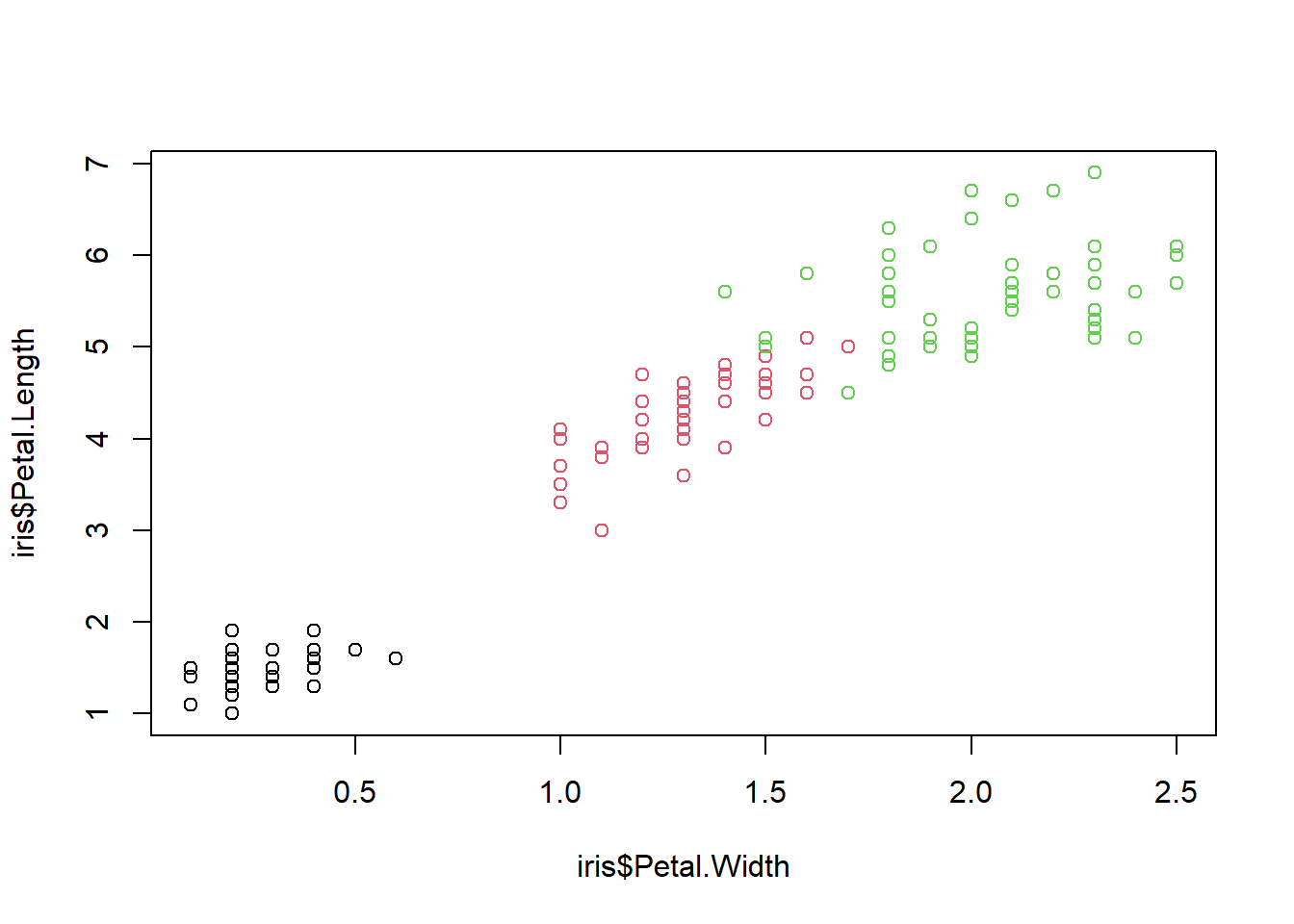

Next, let’s fit a linear model predicting petal length from width and species using lm()

fit1 <- lm(Petal.Length ~ Petal.Width + Species,  data = iris)
summary(fit1)

## 
## Call:
## lm(formula = Petal.Length ~ Petal.Width + Species, data = iris)
## 
## Residuals:
##      Min       1Q   Median       3Q      Max 
## -1.02977 -0.22241 -0.01514  0.18180  1.17449 
## 
## Coefficients:
##                   Estimate Std. Error t value Pr(>|t|)    
## (Intercept)        1.21140    0.06524  18.568  < 2e-16 ***
## Petal.Width        1.01871    0.15224   6.691 4.41e-10 ***
## Speciesversicolor  1.69779    0.18095   9.383  < 2e-16 ***
## Speciesvirginica   2.27669    0.28132   8.093 2.08e-13 ***
## ---
## Signif. codes:  0 '***' 0.001 '**' 0.01 '*' 0.05 '.' 0.1 ' ' 1
## 
## Residual standard error: 0.3777 on 146 degrees of freedom
## Multiple R-squared:  0.9551, Adjusted R-squared:  0.9542 
## F-statistic:  1036 on 3 and 146 DF,  p-value: < 2.2e-16

So what is the equation for this model?

# PL = a + b1*Petal.Width + b2*versicolor + b3*virginica 

Let’s see the intercept and slopes

coefs <- coef(fit1)
coefs

##       (Intercept)       Petal.Width Speciesversicolor  Speciesvirginica 
##          1.211397          1.018712          1.697791          2.276693

Now, let’s create a function that embeds the coefficients into a linear equation

fit1_predict <- function(PW, versicolor, virginica) { 
    Y <- coefs[1] + coefs[2]*PW + coefs[3]*versicolor + coefs[4]*virginica
    print(Y)
}

Test the function with random values for each variable!

fit1_predict(PW=4, versicolor = 0, virginica = 1)

## (Intercept) 
##    7.562937

Compute predictions for different species

preds <- fit1_predict(PW=seq(0,3,by=0.2), versicolor = 0, virginica = 0)   # setosa

##  [1] 1.211397 1.415139 1.618882 1.822624 2.026366 2.230109 2.433851 2.637593
##  [9] 2.841336 3.045078 3.248820 3.452563 3.656305 3.860047 4.063789 4.267532

preds1 <- fit1_predict(PW=seq(0,3,by=0.2), versicolor = 1, virginica = 0)  # versicolor

##  [1] 2.909188 3.112931 3.316673 3.520415 3.724158 3.927900 4.131642 4.335385
##  [9] 4.539127 4.742869 4.946612 5.150354 5.354096 5.557839 5.761581 5.965323

preds2 <- fit1_predict(PW=seq(0,3,by=0.2), versicolor = 0, virginica = 1)  # virginica 

##  [1] 3.488090 3.691833 3.895575 4.099317 4.303060 4.506802 4.710544 4.914287
##  [9] 5.118029 5.321771 5.525513 5.729256 5.932998 6.136740 6.340483 6.544225

# Start with a blank canvas 
plot(NULL, xlim=c(0,3), ylim=c(1,7), 
     xlab="Petal.Width", ylab="Petal.Length")

# Add observed values 
points(Petal.Length ~ Petal.Width, data = iris, col=Species)

# Add predictions 
points(seq(0,3,by=0.2), preds, col=1, pch=19)
points(seq(0,3,by=0.2), preds1, col=2, pch=19)
points(seq(0,3,by=0.2), preds2, col=3, pch=19)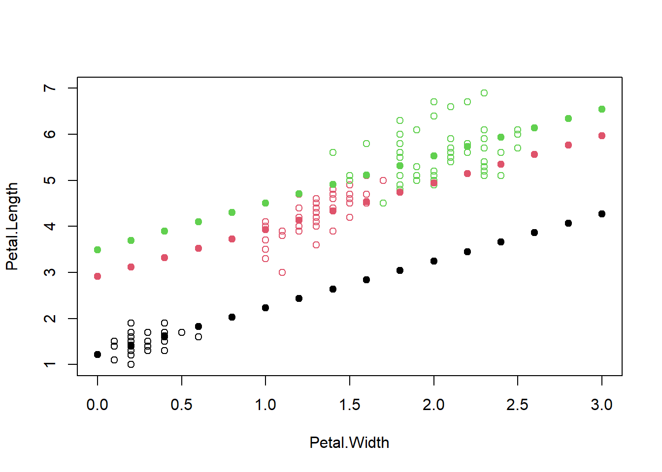

for Loops and Apply Statements

A for loop will perform actions following a sequence or index, for example

x <- 1:10
x

##  [1]  1  2  3  4  5  6  7  8  9 10

for(i in x) { 
    x2 <- i^2
    print(x2)
}

## [1] 1
## [1] 4
## [1] 9
## [1] 16
## [1] 25
## [1] 36
## [1] 49
## [1] 64
## [1] 81
## [1] 100

For example, for loops can be helpful when working with multiple networks

library(igraph)

## 
## Attaching package: 'igraph'

## The following objects are masked from 'package:sna':
## 
##     betweenness, bonpow, closeness, components, degree, dyad.census,
##     evcent, hierarchy, is.connected, neighborhood, triad.census

## The following objects are masked from 'package:network':
## 
##     %c%, %s%, add.edges, add.vertices, delete.edges, delete.vertices,
##     get.edge.attribute, get.edges, get.vertex.attribute, is.bipartite,
##     is.directed, list.edge.attributes, list.vertex.attributes,
##     set.edge.attribute, set.vertex.attribute

## The following objects are masked from 'package:stats':
## 
##     decompose, spectrum

## The following object is masked from 'package:base':
## 
##     union

# simulate network 

par(mfrow=c(1,1)) #Set the plotting dimensions
g <- barabasi.game(n=40, power = 1, directed = F)
plot(g, vertex.label=NA)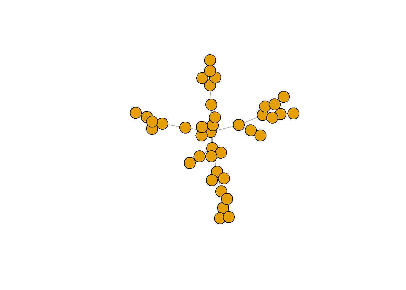

# First, let's use a for loop to create 4 networks with different powers 
pow <- seq(0, 1, length.out=4)
pow

## [1] 0.0000000 0.3333333 0.6666667 1.0000000

# create a container for the networks 
L <- list()

# loop through different values of pow and plot them
set.seed(1)
par(mfrow=c(2,2), mar=c(1,1,1,1))
for(i in seq_along(pow)) {
    
    # simulate preferential attachment
    L[[i]] <- barabasi.game(n=40, power = i, directed = F)
    
    # plot each network
    plot(L[[i]], 
         edge.arrow.size=0.2, 
         vertex.label=NA)
}

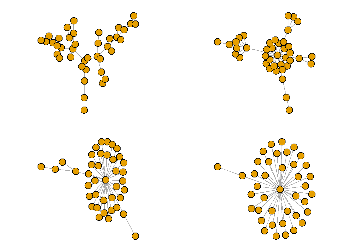
Now we can run some descriptive statistic on the list L One way to do it is to use a loop.

for(i in seq_along(L)) { 
    dens <- graph.density(L[[i]])
    apl <- average.path.length(L[[i]])
    print(c(dens, apl))
}

## [1] 0.050000 4.515385
## [1] 0.050000 2.671795
## [1] 0.050000 2.179487
## [1] 0.050000 1.997436

Sometimes, the same goal can be accomplished more easily by using an apply statement (lapply)

Apply statements take the following form: lapply(list, function)

lapply(L, graph.density)

## [[1]]
## [1] 0.05
## 
## [[2]]
## [1] 0.05
## 
## [[3]]
## [1] 0.05
## 
## [[4]]
## [1] 0.05

# returns a list, so unlist() and put in data frame  
DF <- data.frame(
    Density = unlist(lapply(L, graph.density)),
    APL = unlist(lapply(L, average.path.length))
)
DF

##   Density      APL
## 1    0.05 4.515385
## 2    0.05 2.671795
## 3    0.05 2.179487
## 4    0.05 1.997436

lapply() is used for lists There are also matrix and data.frame versions

For example, apply(array, margin, ...) Or, apply(DF, 2, mean) # this will apply the function mean() to every column