In this post, I will focus on two topics: community detection and subgraph motifs. In previous posts, we have discussed some basic methods for describing network structure. We used these methods to either describe the positioning of individual nodes (e.g., centrality metrics) or some global properties of a network (e.g., connectivity, average path length). Now we will focus on subgraph patterns that transcend the scale of individuals or dyads but nevertheless reside within a global network of interest.
Community detection
Community detection is a method that we can use to identify cluster of nodes that are connected to one another than they are to other parts of the network (Fortunato 2010). We call these communities.
Applications
Identifying communities in networks is a massive area of research. This is because of social media. If companies can detect communities within social media networks, they can use those clusters to target ads, suggest new pages and music to users, and more (Villa, Pasi, and Viviani 2021).
But some us might have similar goals. Suppose we work with a community of land managers who share insights about their project successes and failures. By studying these relationships and identifying communities within them, we may be able to provides insights about who else has similar outcomes. Moreover, dense subgraph communities are examples of echo chambers. We can use these community structures to help our research subjects connect with individuals who may lie outside of their typical partnerships.
Many times, we study networks in which we already have attribute data about group affiliations. In this context, why would we need to use community detection? With community detection we can identify individuals who, despite being affiliated with a specific group, might fall into a different group based on their connections. It also very useful to have “ground truth” data to validate community detection results.
Community detection methods
Community detection uses an algorithm to partition a graph into subgraphs. There are many, many algorithms. Today we’ll focus on some that come packaged in igraph and we will discuss some cutting edge options.
library(igraph)
library(intergraph)
Let’s start by generating a network for our analysis. We’ll do this using statnet.
library(statnet)This little bit of code will generate a network with N nodes and G groups. Edges form based on edge density (ed) within group homophily (h).
# set seed for reproducibility
set.seed(777)
# settings
N = 40 # number of nodes
G = 3 # number of groups
ed = -3 # edge density (log-odds)
h = 2 # group homophily
# empty network
g = network(N, directed = F, density = 0)
# create group attribute
g %v% 'group' = sample(1:G, size = N, replace = T)
# simulate and plot netwok
sim_g = simulate(g ~ edges + nodematch('group'), coef = c(ed,h))
plot(sim_g, vertex.col = g %v% 'group')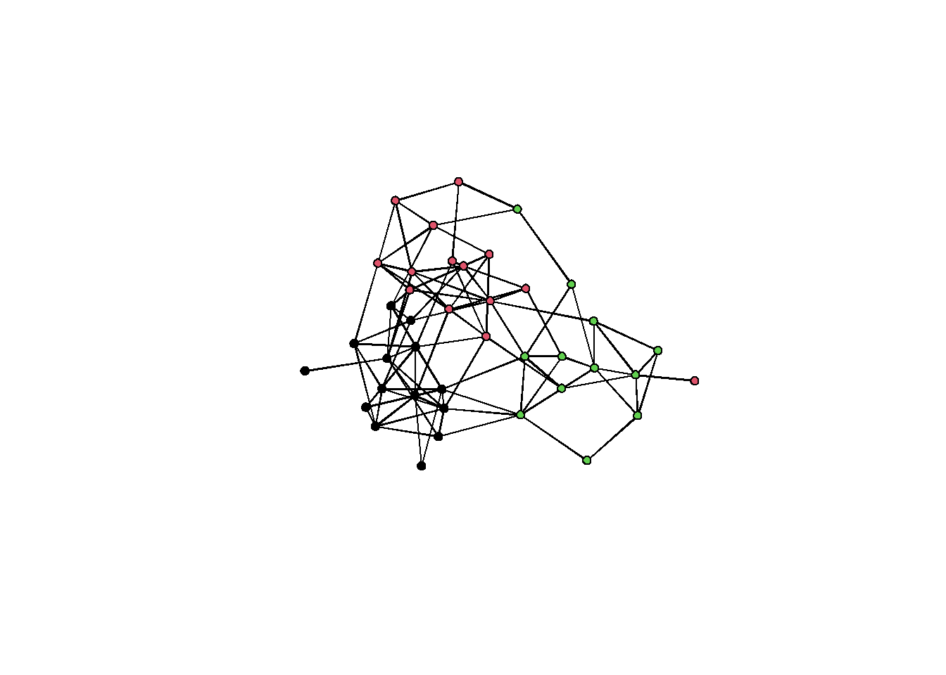 The graph shows some visible clustering. But let’s run some algorithms and what we get.
# convert network to igraph
ig = intergraph::asIgraph(sim_g)
The walktrap algrorithm implements a random walk in which a random origin node is chosen and at each step, the algorithm proceeds randomly to a connected node in the adjacent neighborhood. The documentation suggests that dense communities tend to result in short random walks. This is because in a dense community, a random walk from one node to the next can rapidly take you back to where you began.
clust_wt = cluster_walktrap(ig, steps = 4) # 4 is defaultThe edge_betweeness starts by finding the node with the highest betweenness and then prunes it. This process repeats until it arrives at a rooted tree.
clust_eb = cluster_edge_betweenness(ig)In the louvain algorithm, each node is placed in it’s own community and it then reassigned to a new based on the highest contribution it makes to the overall modularity score of the graph. The resolution parameter controls the number of communities. The default is 1, so I adjust to 0.5 to obtain fewer, albeit larger communities.
clust_lv = cluster_louvain(ig, resolution = 0.55)The leiden algorithm is similar to louvain. It proceeds by reassigned nodes to new groups, partition the graph according to those assignments, and then aggregated them. A key difference is that the leiden algorithm only visits nodes which have a new local neighborhood after the partition and aggregated procedure.
The leiden algorithm currently only works with undirected networks. For directed ones, you would need to use Python or reticulate in R.
clust_ld = cluster_leiden(ig, resolution_parameter = 0.05)Comparing algorithms
Now we can compare the detected communities to those that we originally assigned.
# nmi = normalized mutual information, a conditional entropy calculation
compare(clust_wt, V(ig)$group, method = 'nmi')
## [1] 0.5879944compare(clust_eb, V(ig)$group, method = 'nmi')## [1] 0.6044824compare(clust_lv, V(ig)$group, method = 'nmi')## [1] 0.8393234compare(clust_ld, V(ig)$group, method = 'nmi')## [1] 0.2634199Values closer to 1 indicate that there is a larger difference between the observed groupings and the detected communities. Based on this, we see that the louvain algorithm was the most confused This does not mean that louvain is a worse algorithm – certain algorithms will perform better under different circumstances. The leiden algorithm clear performs the best in this context.
We can also compare the algorithm results to each other.
compare(clust_wt, clust_eb)## [1] 0.6799444compare(clust_wt, clust_lv)## [1] 0.6515201compare(clust_wt, clust_ld)## [1] 1.072275compare(clust_eb, clust_lv)## [1] 0.9575158compare(clust_eb, clust_ld)## [1] 0.8631095compare(clust_lv, clust_ld)## [1] 1.271229Steps and resoluton
Let’s return to the walktrap and leiden algorithms. Recall that I included an additional parameter on these algorithms: steps and resolution. I made a rather arbitrary decision which begs a question: how should we decide how many steps these algorithms should take? Here is one way to help you decide.
In principle, running an algorithm for longer should make it more certain about the number of communities that are in the graph. However, not running it long enough and you will get an inflated number of communities. But this rule of thumb really depends on the algorithm. So let’s cycle through different parameter values and look at how many communities are found.
Begin by setting the largest value we want to test. It is important to go larger than you’d initially expect.
# 100 steps
steps = 100
Create an empty list to store results.
l = list()Then we can use a for loop to run our algorithm multiple times.
for(i in 1:steps) {
    c = cluster_walktrap(ig, steps = i)
    l[[i]] = c$membership
}
Each entry contains a list of membership IDs. If we calculate the number of unique IDs and then take their length, we have the number of communities returned by each run.
n_communties = unlist(lapply(lapply(l, unique), length))Now plot the results against the vector of runs.
plot(1:steps, n_communties, type='o')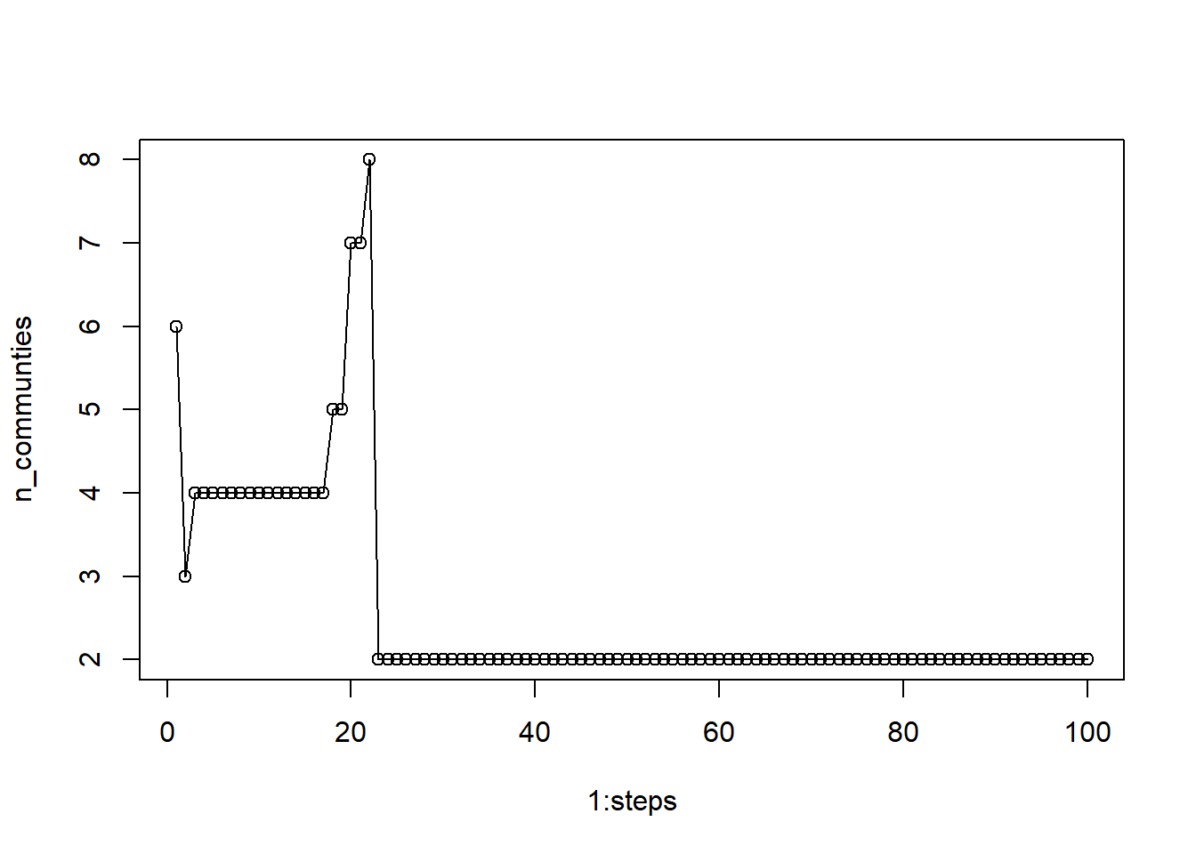 We see that step values under 20 produce more variable numbers of communities. If we chose anything between 5 and 20, we would receive 4 communities, but once we go about 22, the algorithm stabilizes on 2 communities. Any value larger than 22 should be acceptable.
Let’s do the same thing, but for the resolution parameter.
r = seq(0.001,1, length=200)
l = list()
for(i in 1:length(r)) {
    c = cluster_leiden(ig, resolution_parameter = r[i])
    l[[i]] = c$membership
}
n_communties = unlist(lapply(lapply(l, unique), length))
plot(1:length(r), n_communties, type='o')
abline(a=3,b=0, lty=2)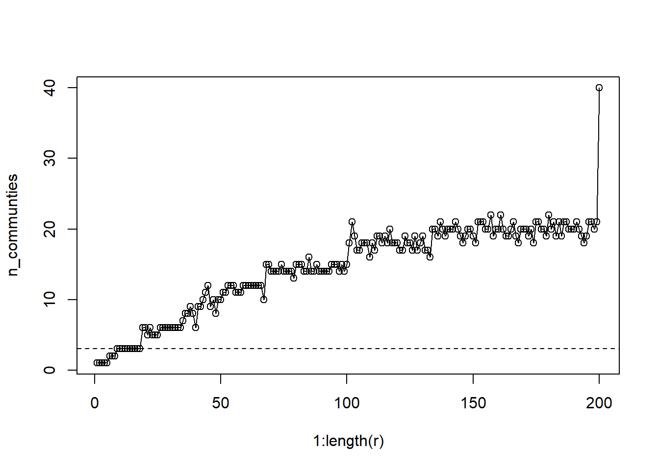
This graph is a bit more complicated. The leiden algorithm is capable of generate up to N communities when the resolution = 1. So how should we decide? Well I’ve plotted a reference line for the number of observed groups. One approach would be to select a resolution that gives that number of groups so that we can compare the placement of nodes in both cases. For other applications, or when no a priori groups are defined, we might opt for additional communities.
r = seq(0.001,1, length=500)
l = list()
for(i in 1:length(r)) {
    c = cluster_louvain(ig, resolution  = r[i])
    l[[i]] = c$membership
}
n_communties = unlist(lapply(lapply(l, unique), length))
plot(1:length(r), n_communties, type='o')
abline(a=3,b=0, lty=2)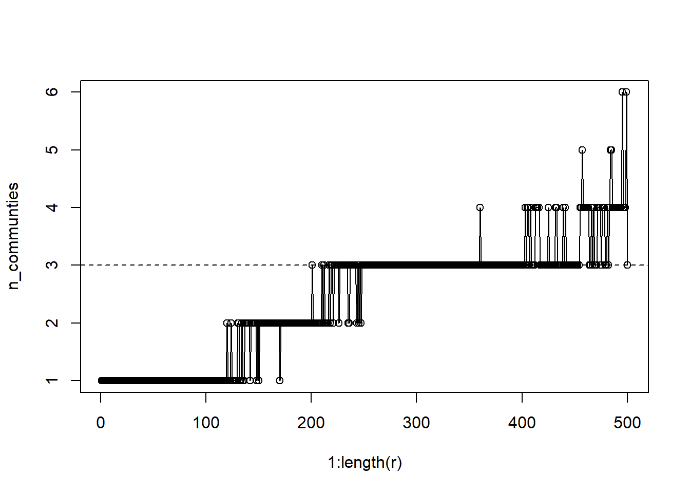
Visualize communities
igraph has built in methods for visualizing the communities that were detected. We can do this by place both the community and the graph in the plot function.
par(mfrow=c(2,3), mar=c(1,1,1,1))
plot(ig,
vertex.color = V(ig)$group,
layout=layout_with_kk,
main='Original')
plot(clust_wt, ig, layout=layout_with_kk, main='Walktrap')
plot(clust_eb, ig, layout=layout_with_kk, main='Edge betweenness')
plot(clust_lv, ig, layout=layout_with_kk, main='Louvain')
plot(clust_ld, ig, layout=layout_with_kk, main='Leiden')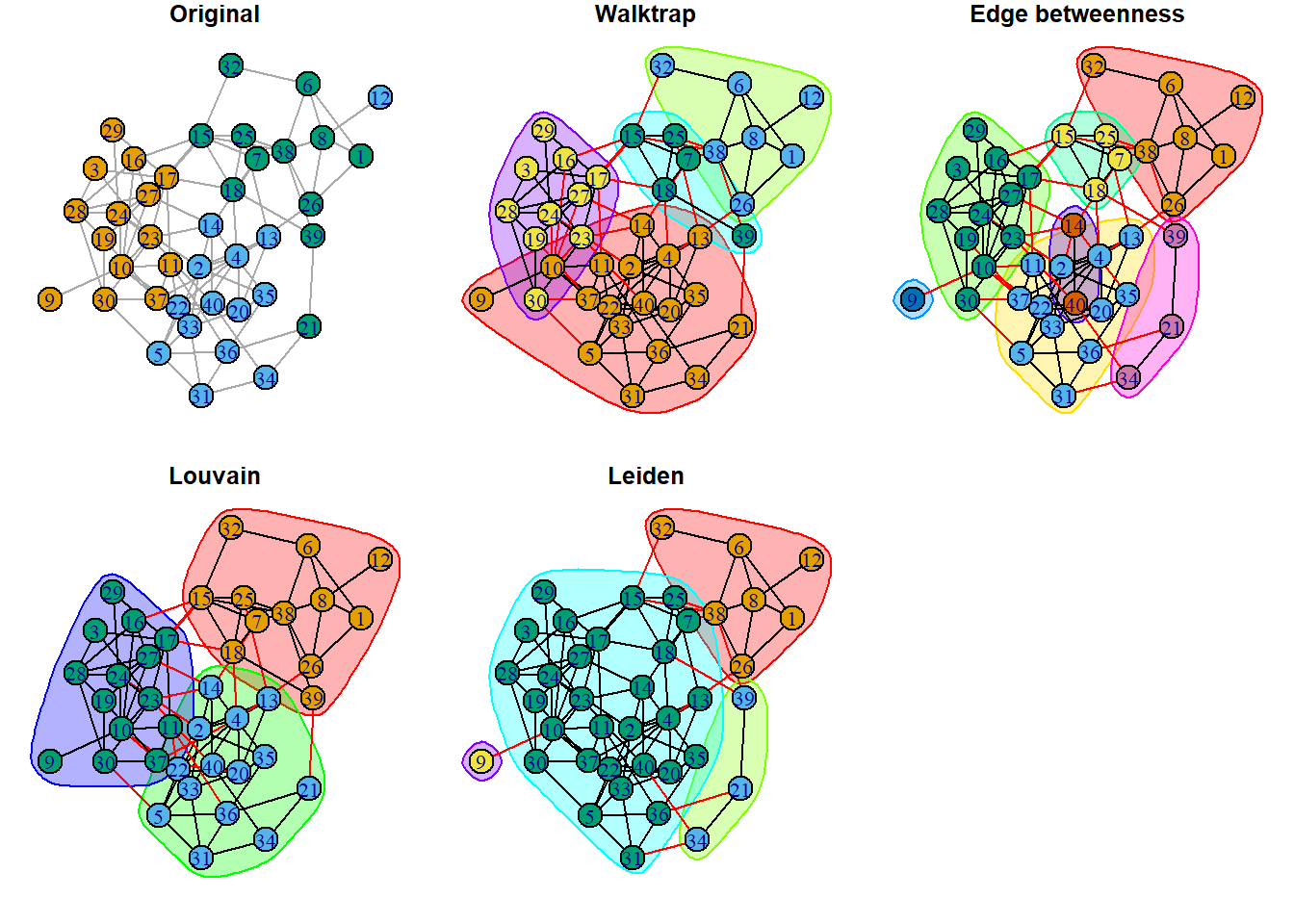 These visuals can be a bit messy, but they do make three things clear:
- Red edges indicate connections between communities, according to the algorithm.
- Bubbles show community boundaries and indicate how many communities were detected. All three algorithms found more communities that observed groups.
- Some nodes fall into multiple bubbles. These indicate nodes that are likely go-betweens.
We can extract memberships from the results and add them graphs. Here is an example from louvain.
par(mfrow=c(1,1))
mem_lv = clust_lv$membership
V(ig)$mem_lv = mem_lv
plot(ig,
     vertex.color = V(ig)$mem_lv,
     layout=layout_with_kk,
     main='Louvain memberships')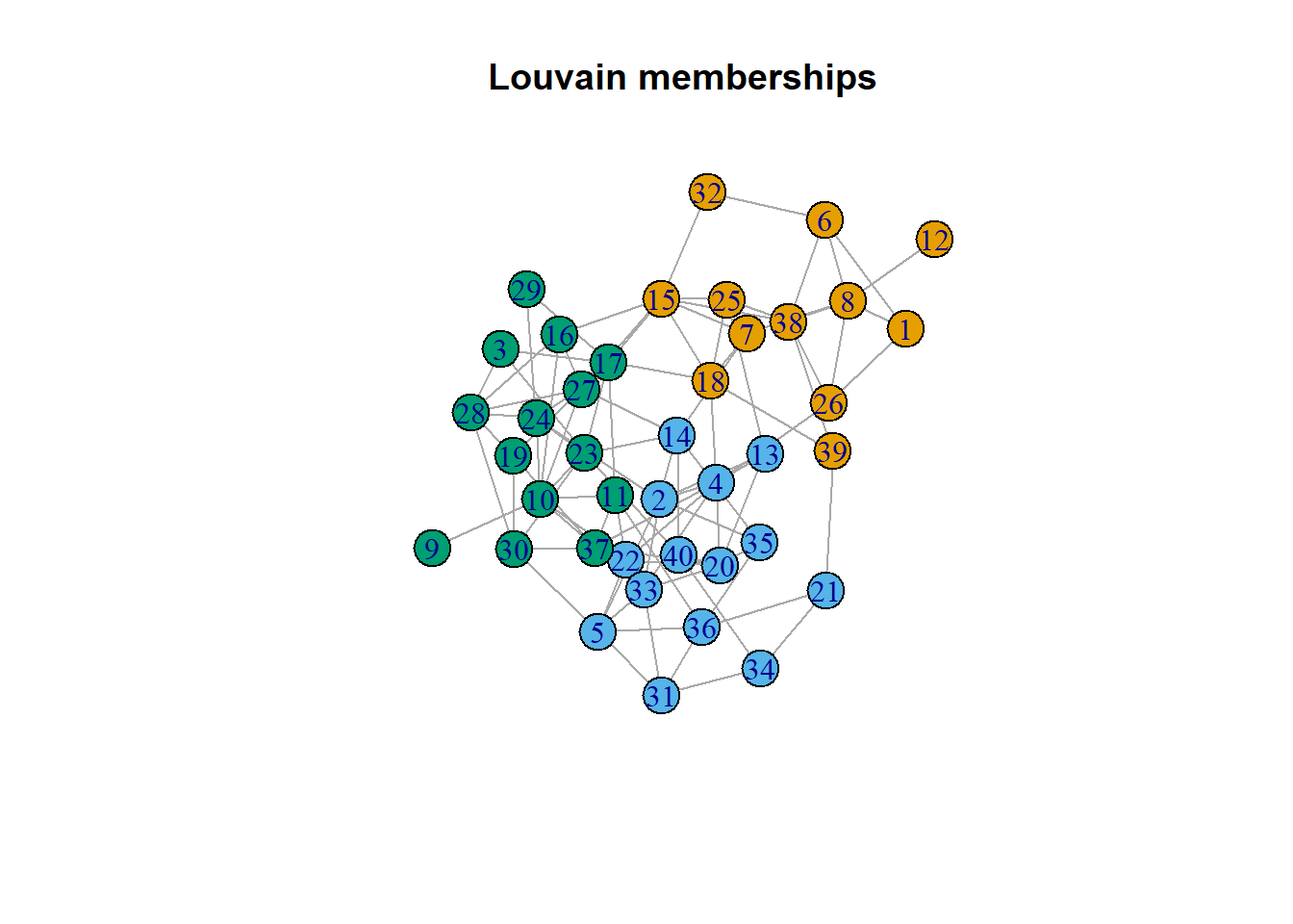
Motifs
Switch gears, let’s talk about motifs. A motif is a specific pattern of nodes and edges. We can think about motifs are structural building blocks that underlie the structure of a network (Bodin and Crona 2009). Our earliest exposure to this idea was when we talked about triads. In an undirected network, there are four possible triads, each representing a different kind of motif.
As we study networks, we may have specific network configurations in mind that are indicative of specific processes. As a cursory comparison, we can thinking about a hierachical star pattern compared to a circlical pattern.
par(mfrow=c(1,2), mar=c(1,1,1,1))
cyc = rbind(c(1,2),c(2,3),c(3,4),c(4,1))
cyc = network(cyc, directed = F)
star = rbind(c(1,2),c(1,3),c(1,4))
star = network(star, directed = F)
gplot(cyc, arrowhead.cex = 0)
gplot(star, arrowhead.cex = 0)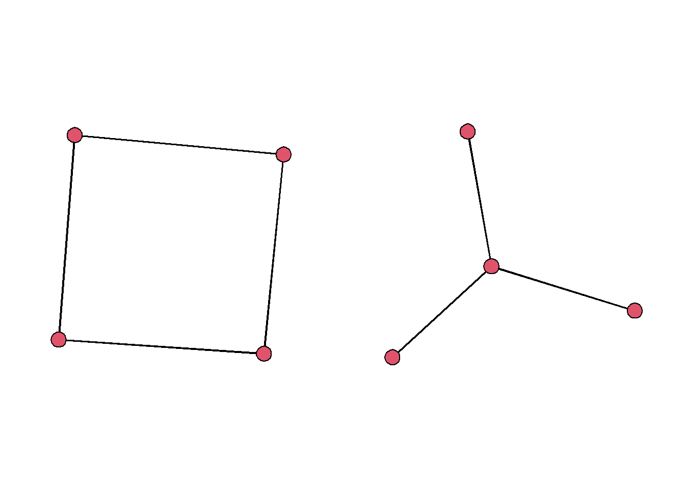 In a structural sense, these two motifs have very different properties. There average path lengths are different and they are less or more centralized with respect to the degree centrality.
centralization(cyc, degree)## [1] 0centralization(star, degree)## [1] 1average.path.length(asIgraph(cyc))## [1] 1.333333average.path.length(asIgraph(star))## [1] 1.5Studying the presence of these motifs within a network might help you understand the social dynamics that are driving the network structure. So how can we do this?
Subgraph isomorphism
Two graphs are said to be isomorphic is they have the same structure, even if the node and edge labels differ. Rarely is it helpful to compare two full networks this way, so most people look for subgraph isomorphisms.
To do this, we specify a subgraph a pattern of interest. Then we can ask 1) whether that pattern is present anywhere in the network, and 2) how many times that pattern occurs. Let’s try this out using the two patterns above as examples.
First, we apply the subgraph_isomorphism function within igraph. This function accepts a specific pattern and a target graph. For anyone who has used grep, this process should seem familiar.
The patterns you provide need to be igraph objects, so let’s check ours.
is.igraph(cyc)## [1] FALSEis.igraph(star)## [1] FALSEThey are not, so we’ll convert them using intergraph.
cyc.ig = asIgraph(cyc)
star.ig = asIgraph(star)
Now let’s plug them in.
subgraph_isomorphic(cyc.ig, ig)## [1] TRUEsubgraph_isomorphic(star.ig, ig)## [1] TRUEThey both exist at least once in the network. Makes a lot sense since these are very generic patterns.
Now can use the same method to identify every set of vertices which are part of one of these two patterns using subgraph_isomorphisms.
cyc.iso = subgraph_isomorphisms(cyc.ig, ig)
star.iso = subgraph_isomorphisms(star.ig, ig)
The function returns a list where every entry is a vertex set. Let’s take a look at the first 6 entries.
head(cyc.iso)## [[1]]
## + 4/40 vertices, from 1527194:
## [1] 1 26 38 6
##
## [[2]]
## + 4/40 vertices, from 1527194:
## [1] 1 26 38 8
##
## [[3]]
## + 4/40 vertices, from 1527194:
## [1] 1 8 38 26
##
## [[4]]
## + 4/40 vertices, from 1527194:
## [1] 1 8 38 6
##
## [[5]]
## + 4/40 vertices, from 1527194:
## [1] 1 6 38 8
##
## [[6]]
## + 4/40 vertices, from 1527194:
## [1] 1 6 38 26head(star.iso)## [[1]]
## + 4/40 vertices, from 1527194:
## [1] 1 26 6 8
##
## [[2]]
## + 4/40 vertices, from 1527194:
## [1] 1 26 8 6
##
## [[3]]
## + 4/40 vertices, from 1527194:
## [1] 1 8 26 6
##
## [[4]]
## + 4/40 vertices, from 1527194:
## [1] 1 8 6 26
##
## [[5]]
## + 4/40 vertices, from 1527194:
## [1] 1 6 8 26
##
## [[6]]
## + 4/40 vertices, from 1527194:
## [1] 1 6 26 8One thing we can do is count them up.
length(cyc.iso)## [1] 624length(star.iso)## [1] 3876We find there are many more stars then that are cycles. A simple reason for this is that there is one addition edge in a cycle.
If we used induced = T, then the resulting list will contain new subgraph objects. This is helpful if you wish to plot every subgraph.
cyc.iso = subgraph_isomorphisms(cyc.ig, ig, induced = T)
star.iso = subgraph_isomorphisms(star.ig, ig, induced = T)
Another cool feature of these functions is the ability to specify domains – these are specific subsets of vertices that we can use to constrain the search for isomorphisms. To try this out, let’s use a slightly more complicated pattern.
First we want to isolate a set of vertices to search. We can do this using the group attribute.
group1 = V(ig)$vertex.names[ V(ig)$group == 1 ]
group2 = V(ig)$vertex.names[ V(ig)$group == 2 ]
group3 = V(ig)$vertex.names[ V(ig)$group == 3 ]
Now we construct a list that labels each group set as a domain.
domains = list(`1` = group1,
               `2` = group2,
               `3` = group3)
I’m going simulate a small graph using a preferential attachment simulation. We need a separate attachment simulation for each group because the pattern must be of the same size as the domain of interest.
set.seed(777)
pa1 = barabasi.game(length(group1), power = 2, directed = F)
pa2 = barabasi.game(length(group2), power = 2, directed = F)
pa3 = barabasi.game(length(group3), power = 2, directed = F)
par(mfrow=c(1,3), mar=c(1,1,1,1))
plot(pa1)
plot(pa2)
plot(pa3)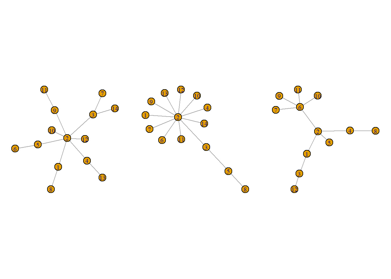 I suspect it is very unlikely that we will find these networks in our domains but let’s proceed.
Then we run the function as before with the domains object included.
iso1 = subgraph_isomorphisms(pattern = pa1,
                             target = ig,
                             domains = domains)
***I haven’t been able to get this code to run properly so I am still debugging, but this is the general process.
Parting thoughts
Community detection
This cursory introduction shows us how to use communtity detection, some specific applications, and a general workflow. But there are many algorithms to explore. For example, we have at all discussed deep learning or neural networks. These are possible topics for future meetings.
IF you want to learn more, I noticed there are several recent preprints that discuss these topics.
Motifs
We have hardly scratched the surface of motifs. Mostly due to a lack of time. But one package you may want to check out is motifr. This package assists with motif analysis, particular in multilevel/multilayer networks.