Preamble
We’ve talked about ERGMs but we really only covered binary ERGMs. Not too long ago, binary ERGMs were all that was available to us in R, something that anthropologist David Nolin noted in a 2010 paper on food sharing in Human Nature:
“The chief disadvantage of ERGM is that dependent-variable networks can consist only of binary ties… Networks composed of valued ties can be binarized for use with ERGM, but this entails a loss of statistical information.”
We no longer have this problem. Instead, we have a plethora of extensions and alternatives, particularly for edges that consist of count data. Any of these packages could work: ergm.count, STRAND, the social relations model (Kenny and LaVoie 1984), GERGM, bergm, latentnet, etc.
Let’s stick with the statnet suite that we started with and look at valued ergms using the ergm.count package. A published article by Martina Morris and Pavel Krivitsky (2017) accompanies this package, and there is also a very helpful workshop on the statnet website.
The other thing we will do today is spend a little time looking at the MCMC control settings in the ERGM package. When it comes to MCMC and MLE controls, there is a lot to cover. We will be focusing on some of the most commonly adjusted settings when calibrating an MCMC sampler. For a more interactive look at MCMC algorithms, check out these simulations.
Setup
For this example, let’s use the network data from Koster and Leckie (2014) that is included as part of the rethinking package.
data('KosterLeckie', package = 'rethinking')Now let’s load up statnet.
library(statnet)Wrangling
The KosterLeckie data contains information about 25 households (kl_households) and their food sharing relationships (kl_dyads). These relations are stored in a dyadic format. Take a look.
head(kl_dyads)## hidA hidB did giftsAB giftsBA offset drel1 drel2 drel3 drel4 dlndist dass
## 1 1 2 1 0 4 0.000 0 0 1 0 -2.790 0.000
## 2 1 3 2 6 31 -0.003 0 1 0 0 -2.817 0.044
## 3 1 4 3 2 5 -0.019 0 1 0 0 -1.886 0.025
## 4 1 5 4 4 2 0.000 0 1 0 0 -1.892 0.011
## 5 1 6 5 8 2 -0.003 1 0 0 0 -3.499 0.022
## 6 1 7 6 2 1 0.000 0 0 0 0 -1.853 0.071
## d0125
## 1 0
## 2 0
## 3 0
## 4 0
## 5 0
## 6 0So we’ll have to do just a little bit of wrangling to get this into an edgelist format. First, we isolate the AB columns along with the household IDs.
AB_dyads = kl_dyads[, c('hidA','hidB','giftsAB')]Then we want to do the same thing, but we need to switch the order of the hidA and hidB column so that they exhibit the correction directionality.
BA_dyads = kl_dyads[, c('hidB','hidA','giftsBA')]Now we will rename the columns, bind them together, and filter out any rows where there were no gifts exchanged.
# rename
colnames(AB_dyads) = c('sender','receiver','gifts')
colnames(BA_dyads) = c('sender','receiver','gifts')
# filter and bind
el = rbind(AB_dyads[ !AB_dyads$gifts == 0, ],
           BA_dyads[ !BA_dyads$gifts == 0, ])
Edge attributes can be stored in an edgelist as additional columns. So in this case, we have an edgelist with a single edge attribute called gifts. Let’s construct the full network now. Let’s not forget to add the vertex attributes from the kl_households file.
g = network(el, vertex.attr = kl_households)
g
## Network attributes:
## vertices = 25
## directed = TRUE
## hyper = FALSE
## loops = FALSE
## multiple = FALSE
## bipartite = FALSE
## total edges= 427
## missing edges= 0
## non-missing edges= 427
##
## Vertex attribute names:
## hfish hgame hid hpastor hpigs hwealth vertex.names
##
## Edge attribute names:
## giftsLet’s quickly visualize this network.
library(tidygraph)
library(ggraph)

g %>% as_tbl_graph() %>%
    ggraph() +
    geom_edge_link(aes(width=gifts))
# Questions
First, let’s decide some specific questions that we wanted to ask about this network. In particular, I would like to know the following:
- Is reciprocity a strong driver of edge formation?
- What impact does harvest size have on the number of gives and sharing partners a household has?
- How prevalent are triangles in this network?
Constructing a model
Building a ERGM that can handle edge counts is very similar to how we constructed our ERGMs before. Many of the functions are the same – ergm, simulate, summary – as is the general syntax for including covariates.
If you check the documentation for ergm-terms, you’ll find that each term has a listed of network types that it is compatible with: binary, directed, undirected, valued, etc. This helps us find the valued versions of particular terms.
For example, in a binary ERGM we include an edges term that estimates the overall edge density. However, the density of a valued ERGM cannot be described solely by the number of observed edges, because the values on the edges are relevant. According to the documentation, a threshold can be set, but in some cases there may not be an obvious maximum value for the edges, making it impossible to calculate a density. Instead, we include a sum term in place of the edges term.
We can test this by taking a summary of g ~ sum – a simple valued ERGM.
summary(g ~ sum)## Error: ERGM term 'sum' function 'InitErgmTerm.sum' not found.Oops we’re getting an error!
This is because there is another key difference between valued and binary ERGMs. A valued ERGM requires that a response argument be included in the ERGM function. This “response” is the valued edge attribute that we want to estimate in the model (i.e., gifts).
summary(g ~ sum, response = 'gifts')## sum
## 2871This summary tells us the sum of all values across every edge in the network. We can validate this.
sum(el$gifts)## [1] 2871Reference distribution
In a binary ERGM, ties are either present or absent. Under the hood, this data structure implies a very specific reference distribution – a Bernoulii distribution. You can think of a Bernoulli kind of like a weighted coin flip where the probability tells us how likely we are to get a 1. The Bernoulli is the same as a Binomial distribution that has size = 1.
# binomial with same number of edges as network
rbinom(n=427, size=1, prob=0.5)
## [1] 0 0 1 1 0 0 1 0 1 1 0 1 0 0 1 1 0 0 0 1 1 0 0 1 1 1 0 0 1 0 0 1 1 1 0 1 1
## [38] 1 0 0 0 0 0 1 1 0 0 1 0 1 0 0 1 0 1 0 0 1 1 0 0 0 0 0 0 0 0 0 0 1 1 0 0 0
## [75] 0 0 1 0 1 1 1 0 1 0 1 1 1 0 0 0 0 1 1 1 1 1 1 1 1 1 0 0 1 0 0 1 0 0 0 1 0
## [112] 0 0 1 1 0 1 1 0 1 1 0 1 0 1 1 0 1 1 1 0 0 0 0 0 1 1 1 0 1 1 0 1 1 0 1 0 1
## [149] 0 1 1 1 0 0 1 1 1 0 0 0 1 1 0 0 0 0 0 1 0 1 1 1 0 0 1 0 1 1 0 0 1 0 0 0 1
## [186] 0 0 0 0 0 1 0 0 1 0 0 0 1 0 1 0 0 0 0 1 1 0 1 0 1 1 0 0 1 1 0 0 0 0 1 1 0
## [223] 1 1 1 0 0 1 0 1 1 1 0 0 0 1 1 1 0 1 0 0 1 1 1 1 1 1 1 0 1 1 1 0 0 1 0 1 0
## [260] 1 1 1 0 1 1 1 0 0 0 1 0 0 0 1 0 1 1 1 1 1 0 1 1 0 0 0 1 0 0 0 1 1 0 0 0 0
## [297] 1 0 0 0 1 0 0 0 0 0 0 1 1 0 0 1 1 0 1 0 0 0 0 0 0 0 0 0 0 1 0 0 1 0 0 0 1
## [334] 0 0 0 0 0 0 0 0 0 1 1 1 0 1 0 0 0 1 1 0 0 1 0 0 0 1 1 0 0 1 0 0 0 0 0 0 0
## [371] 1 0 1 0 0 0 0 0 1 0 0 1 1 0 0 1 0 1 1 0 0 0 1 0 0 1 1 1 1 1 0 1 1 1 0 1 1
## [408] 1 0 0 1 1 0 1 1 1 0 1 1 1 0 1 0 0 1 0 1For a valued ERGM, it isn’t totally obvious what the reference distribution should be since there are multiple distributions that can be used for counts and continuous values. Let’s check the documentation using help("ergm-references").
We find that ergm.count supports three types of reference distributions: Poisson, Geometric, and Binomial. We need to choose a reference distribution that is sensible for our gift data.
hist(g %e% 'gifts')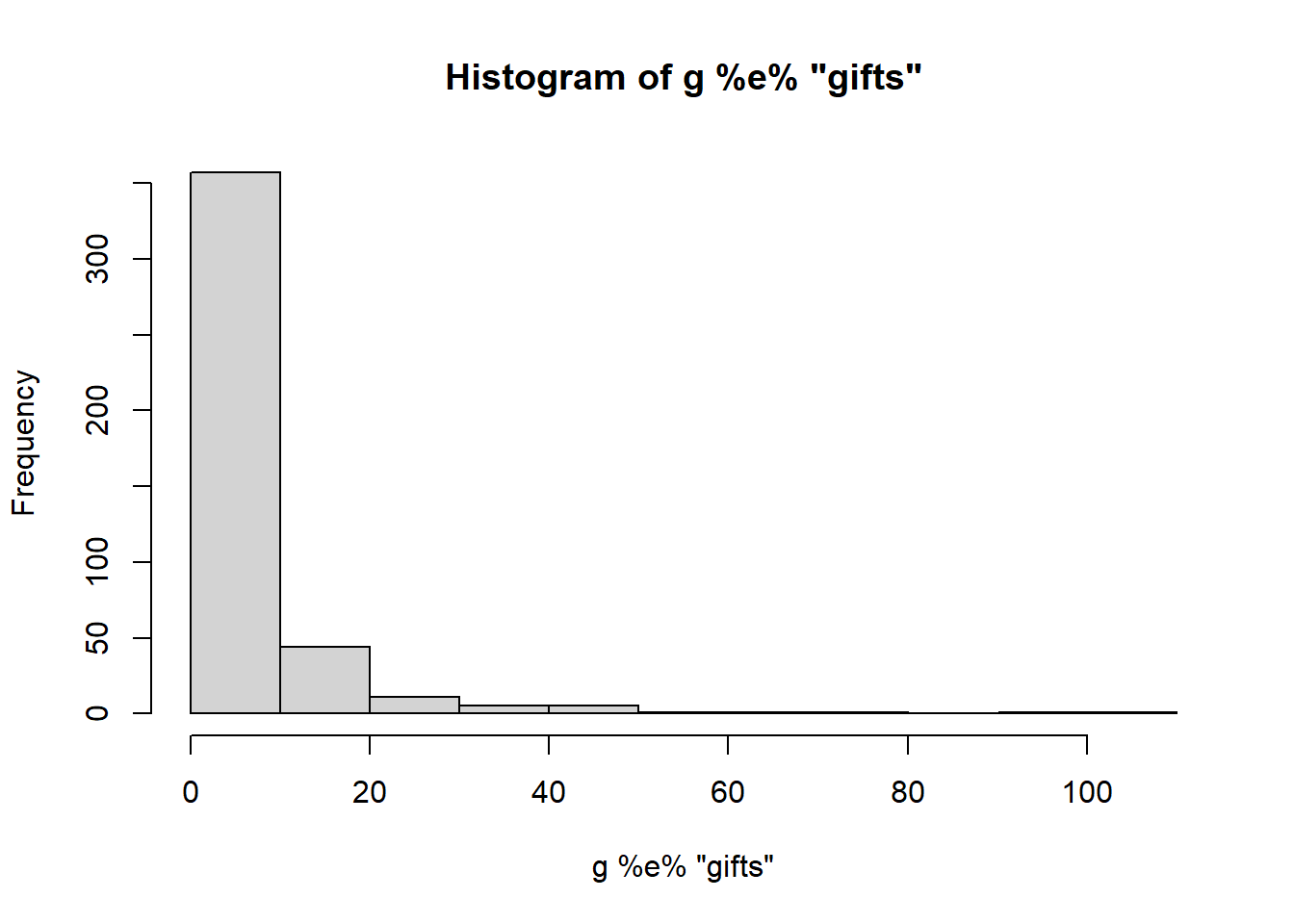
We have a long tail and a high number of zeros. Let’s explore these other distributions and see if they are similar.
Poisson
A poisson distribution is a discrete distribution whose mean and variance are described by a single parameter lambda.
hist(rpois(n=427, lambda = 1))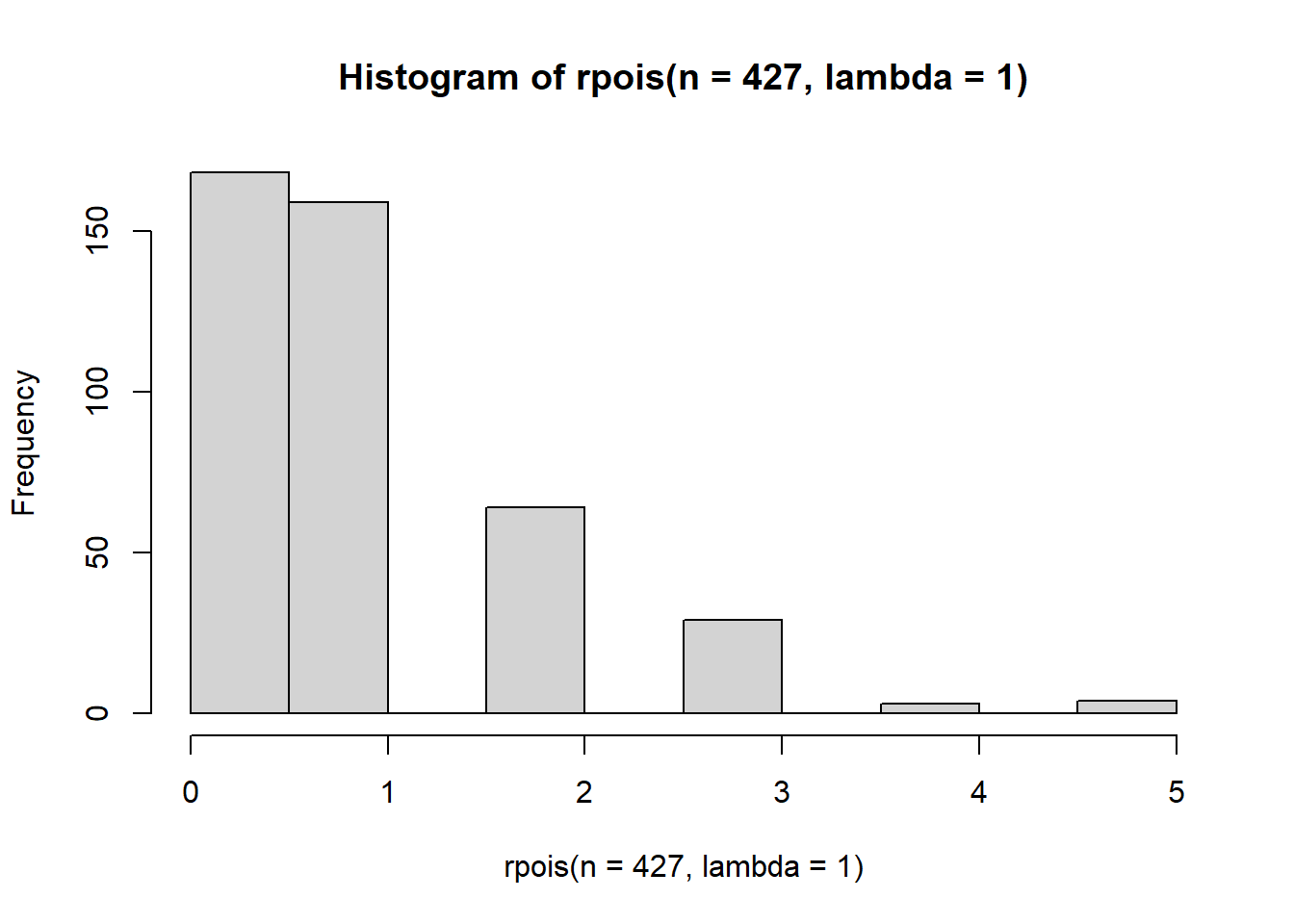
Higher values of lambda will lead to a more bell shaped curve.
hist(rpois(n=427, lambda = 10))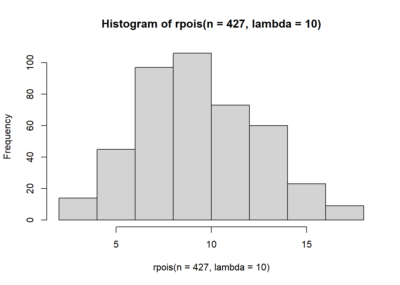 This is quite what we’re after since our gift distribution has a lot of zeros. Perhaps we could try a zero-inflated Poisson, an option that is supported by the
 ergm.count package. I’m constructing this distribution as a mixture of a bernoulli (for the zeros) and a poisson.
hist( ifelse(rbinom(n=427,size=1,prob=0.5) == 0, 0 , rpois(n=427, lambda=2)),
main = '')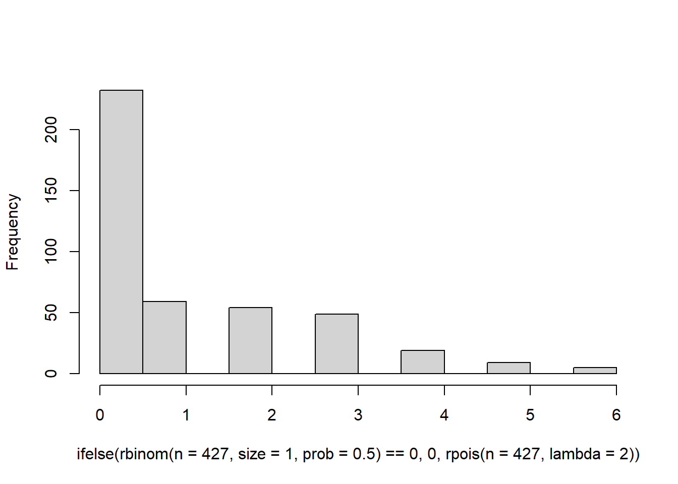 This is a bit closer, but the problem is that we don’t have a long enough tail. Our data ranges all the way up to 100. Increasing the value of lambda won’t help either because it will lead to a hurdle distribution. See here.
hist( ifelse(rbinom(n=427,size=1,prob=0.5) == 0, 0 , rpois(n=427, lambda=10)),
      main = '')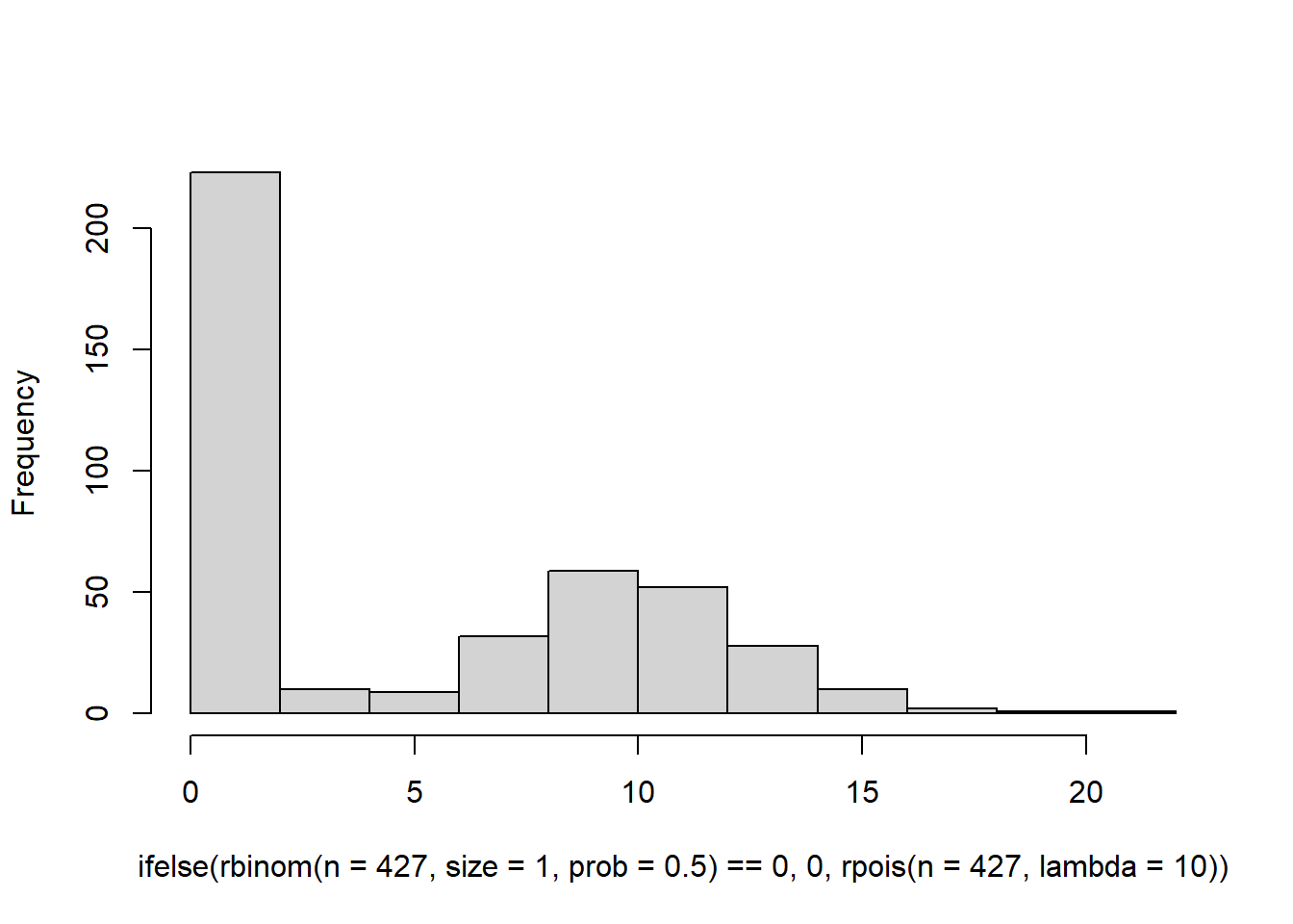
Binomial
The Binomial distribution may work if we weight the probability toward low values and set a high value of size. We should use the maximum value of gifts that is observed in the network.
max(el$gifts)## [1] 110hist(rbinom(n=427, size=max(el$gifts), prob = 0.01))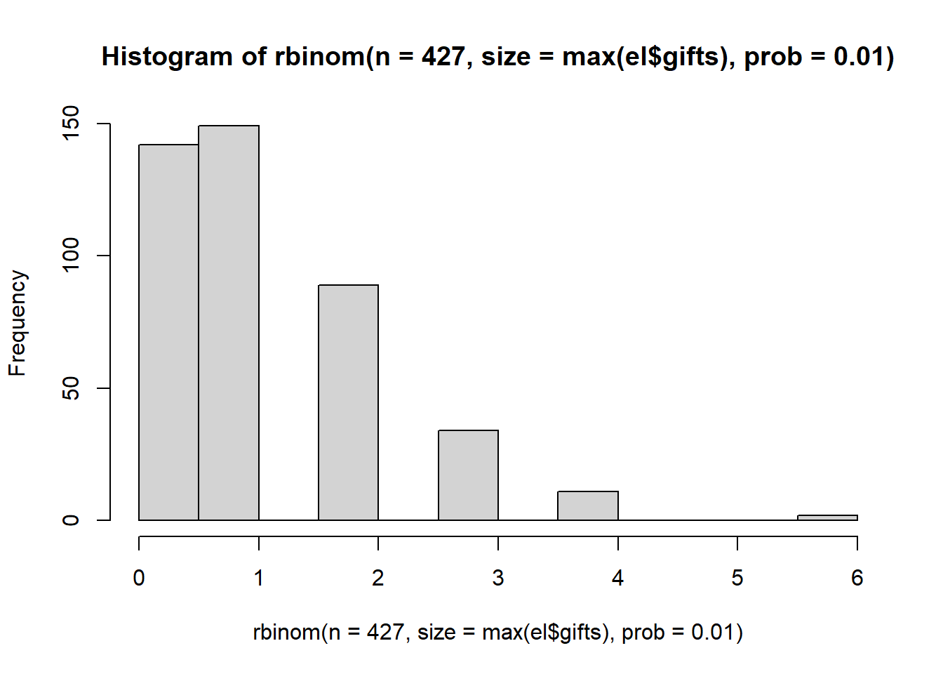
We’ve having the same problem as the poisson distribution. and In fact, the Poisson and Binomial distribution because one and the same when there is a high count.
Geometric
Our last option is the geometric distribution. The geometric distribution is described by a single parameter prob which controls the “probability of success”. When prob is near 1, the distribution collapses onto a small number of values and a short tail.
hist(rgeom(n=427, prob=0.9))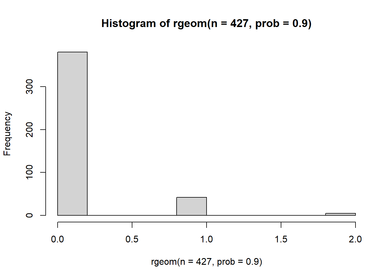 But when probability is low, the distribution exhibits a much longer tail and an inflation of low values.
hist(rgeom(n=427, prob=0.1))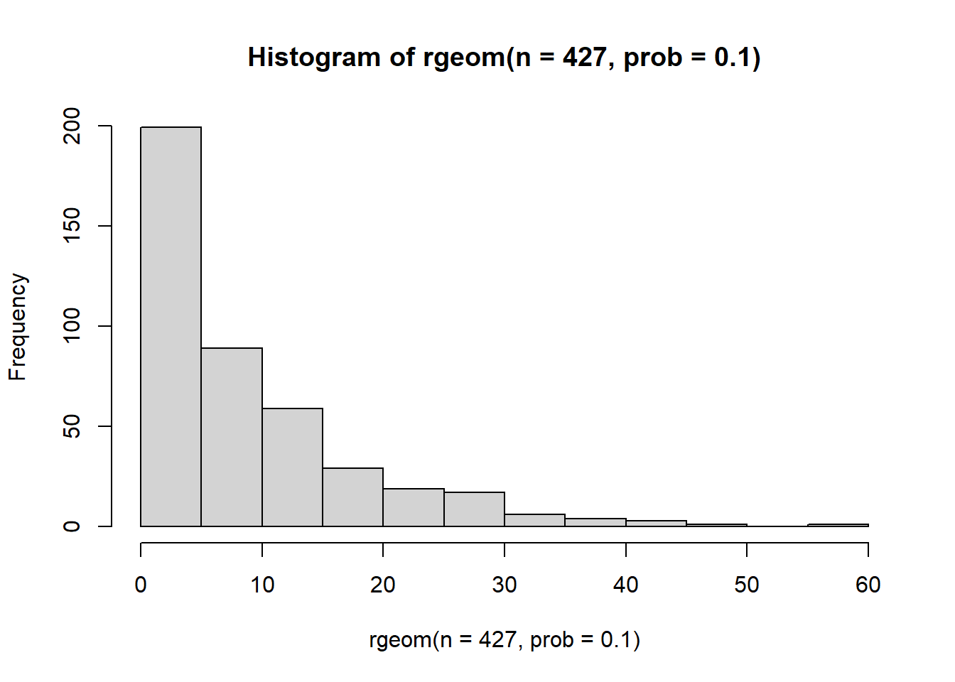
This seems much closer to the kind of reference distribution we are looking for. Let’s give it a try.
fit0 = ergm(g ~ sum, response = 'gifts', reference = ~Geometric)## Best valid proposal 'Geometric' cannot take into account hint(s) 'sparse'.## Starting contrastive divergence estimation via CD-MCMLE:## Iteration 1 of at most 60:## Convergence test P-value:3.9e-12## The log-likelihood improved by 0.4016.## Iteration 2 of at most 60:## Convergence test P-value:1.8e-08## The log-likelihood improved by 0.1277.## Iteration 3 of at most 60:## Convergence test P-value:4.6e-02## The log-likelihood improved by 0.01478.## Iteration 4 of at most 60:## Convergence test P-value:7.2e-04## The log-likelihood improved by 0.03908.## Iteration 5 of at most 60:## Convergence test P-value:6.1e-02## The log-likelihood improved by 0.01288.## Iteration 6 of at most 60:## Convergence test P-value:1.7e-03## The log-likelihood improved by 0.03562.## Iteration 7 of at most 60:## Convergence test P-value:3.3e-02## The log-likelihood improved by 0.01704.## Iteration 8 of at most 60:## Convergence test P-value:8.8e-01## Convergence detected. Stopping.## The log-likelihood improved by < 0.0001.## Finished CD.## Starting Monte Carlo maximum likelihood estimation (MCMLE):## Iteration 1 of at most 60:## Optimizing with step length 0.3570.## The log-likelihood improved by 2.5646.## Estimating equations are not within tolerance region.## Iteration 2 of at most 60:## Optimizing with step length 0.3951.## The log-likelihood improved by 1.8599.## Estimating equations are not within tolerance region.## Iteration 3 of at most 60:## Optimizing with step length 0.7296.## The log-likelihood improved by 2.5740.## Estimating equations are not within tolerance region.## Iteration 4 of at most 60:## Optimizing with step length 1.0000.## The log-likelihood improved by 0.1594.## Estimating equations are not within tolerance region.## Iteration 5 of at most 60:## Optimizing with step length 1.0000.## The log-likelihood improved by 0.0008.## Convergence test p-value: 0.0004. Converged with 99% confidence.
## Finished MCMLE.
## Evaluating log-likelihood at the estimate. Setting up bridge sampling...
## Best valid proposal 'Geometric' cannot take into account hint(s) 'sparse'.
## Using 16 bridges: 1 2 3 4 5 6 7 8 9 10 11 12 13 14 15 16 .
## Note: Null model likelihood calculation is not implemented for valued
## ERGMs at this time. This means that all likelihood-based inference
## (LRT, Analysis of Deviance, AIC, BIC, etc.) is only valid between
## models with the same reference distribution and constraints.
## This model was fit using MCMC. To examine model diagnostics and check
## for degeneracy, use the mcmc.diagnostics() function.summary(fit0)## Call:
## ergm(formula = g ~ sum, response = "gifts", reference = ~Geometric)
##
## Monte Carlo Maximum Likelihood Results:
##
## Estimate Std. Error MCMC % z value Pr(>|z|)
## sum -0.188961 0.008011 0 -23.59 <1e-04 ***
## ---
## Signif. codes: 0 '***' 0.001 '**' 0.01 '*' 0.05 '.' 0.1 ' ' 1
##
## Null Deviance: 0 on 600 degrees of freedom
## Residual Deviance: -4057 on 599 degrees of freedom
##
## Note that the null model likelihood and deviance are defined to be 0.
## This means that all likelihood-based inference (LRT, Analysis of
## Deviance, AIC, BIC, etc.) is only valid between models with the same
## reference distribution and constraints.
##
## AIC: -4055 BIC: -4051 (Smaller is better. MC Std. Err. = 59.79)Good news is that the model runs. Let’s worry about interpetation a bit later.
Question 1
Let’s build a model to answer question 1 about the effects of reciprocity. In our last workshop, we used the mutual term to estimate reciprocity. In that scenario, it’s pretty straight forward: reciprocity occurs when there is both an edge from \(i \rightarrow j\) and \(j \rightarrow i\).
In the valued case, it isn’t so simple. Maybe there is an edge from \(i \rightarrow j\) with a value of 1, but the value of the edge from \(j to i\) has a value of 10. Is this truly reciprocity or do the values need to be the same? The answer isn’t obvious and you should consult your ethnographic information about the study system to make a decision.
If we consult the help("ergm-terms") documentation, we find that mutual terms for valued networks require additional arguments form. We have the following options:
min= mutual pairs match based on the minimum value observed (easy to interpret)nabsdiff= mutual pairs match based on the absolute difference between themproduct= mutual pairs match using product of edge valuesgeometric= mutual pairs form an uncentered covariance (hard to interpret)
There is no clear answer here. I am going to choose nabsdiff because this will allow us to keep information about both the differences between edge values and their overall combination.
fit1.1 = ergm(g ~ sum + mutual(form="nabsdiff"), response = 'gifts', reference = ~Geometric)
summary(fit1.1)
## Call:
## ergm(formula = g ~ sum + mutual(form = "nabsdiff"), response = "gifts",
## reference = ~Geometric)
##
## Monte Carlo Maximum Likelihood Results:
##
## Estimate Std. Error MCMC % z value Pr(>|z|)
## sum -0.22147 0.01313 0 -16.87 < 1e-04 ***
## mutual.nabsdiff -0.05487 0.01704 0 -3.22 0.00128 **
## ---
## Signif. codes: 0 '***' 0.001 '**' 0.01 '*' 0.05 '.' 0.1 ' ' 1
##
## Null Deviance: 0 on 600 degrees of freedom
## Residual Deviance: -4034 on 598 degrees of freedom
##
## Note that the null model likelihood and deviance are defined to be 0.
## This means that all likelihood-based inference (LRT, Analysis of
## Deviance, AIC, BIC, etc.) is only valid between models with the same
## reference distribution and constraints.
##
## AIC: -4030 BIC: -4021 (Smaller is better. MC Std. Err. = 41.26)The results of this model indicate that there is a significant but slightly negative effect of mutuality on this network. A good practice would be to try other forms of mutuality and determine if some of wildly different than the others. I did this already and they all give similar results.
Question 2
For the next question, I want to understand how harvests of fish and game influence connections. First, I need to combined the hgame and hfish into on node attributes.
g %v% 'harv' = g %v% 'hgame' + g %v% 'hfish'Now I need to choose the appropriate ERGM term: nodecov. Like the mutual term we have to specify additional arguments. In this case, we want to base our node covariate term on the sum of the the edges connected to the household.
fit2.1 = ergm(g ~ sum + nodecov(attr='harv', form='sum'), response = 'gifts', reference = ~Geometric)
summary(fit2.1)
## Call:
## ergm(formula = g ~ sum + nodecov(attr = "harv", form = "sum"),
## response = "gifts", reference = ~Geometric)
##
## Monte Carlo Maximum Likelihood Results:
##
## Estimate Std. Error MCMC % z value Pr(>|z|)
## sum -0.243765 0.012306 0 -19.809 <1e-04 ***
## nodecov.sum.harv 0.020437 0.002556 0 7.995 <1e-04 ***
## ---
## Signif. codes: 0 '***' 0.001 '**' 0.01 '*' 0.05 '.' 0.1 ' ' 1
##
## Null Deviance: 0 on 600 degrees of freedom
## Residual Deviance: -4119 on 598 degrees of freedom
##
## Note that the null model likelihood and deviance are defined to be 0.
## This means that all likelihood-based inference (LRT, Analysis of
## Deviance, AIC, BIC, etc.) is only valid between models with the same
## reference distribution and constraints.
##
## AIC: -4115 BIC: -4106 (Smaller is better. MC Std. Err. = 45.06)Now the results show that there is a very slight but significant effect of harvests the number incoming and outgoing connections a household has. In the binary case, we can interpret this as is, but in the valued case, we may want to determine what the probability is for a specific edge value. To do this, we need to multiply our coefficient estimates of sum and nodecov by values of interest.